Grønlandsudvalget 2011-12, Forsvarsudvalget 2011-12
GRU Alm.del Bilag 23, FOU Alm.del Bilag 171
Offentligt
Spatial statistical analysis of contamination241239level of Am and PuThule, North-West Greenland
Jens Strodl Andersen, JSA EnviroStatRisø-R-1791(EN)October 2011
Risø-R-Report
Author:Jens Strodl Andersen, JSA EnviroStatTitle:Spatial statistical analysis of contamination239
level of
241
Am and
Risø-R-1791(EN)October 2011
Pu, Thule, North-West Greenland
Abstract
A spatial analysis of data on radioactive pollution on land at Thule,North-West Greenland is presented. The data comprises levels of241241Am and239,240Pu on land.Maximum observed level of Am
ISSN 0106-2840ISBN 978-87-550-3933-9
is 2.8×10⁵Bq m-2. Highest levels were observed nearNarsaarsuk. This area was also sampled most intensively. InGrønnedal the maximum observed level of241Am is 1.9×10⁴Bq m-2. Prediction of the overall amount of241Am and239,240Pu is based on grid points within the range from thenearest measurement location. The overall amount istherefore highly dependent on the model. Under the optimalspatial model for Narsaarsuk, within the area of prediction,the predicted total amount of241Am is 45 GBq and thepredicted total amount of239,240Pu is 270 GBq.
Contract no.:
Group's own reg. no.:
Sponsorship:
Cover :
Pages:73Tables: 24References: 50Information Service DepartmentRisø National Laboratory forSustainable EnergyTechnical University of DenmarkP.O.Box 49DK-4000 RoskildeDenmarkTelephone +45 46774005[email protected]Fax +45 46774013www.risoe.dtu.dk
Contents122.12.22.32.42.53Geographic location of the measurementsStatistical methodsLikelihood based parameter estimationValidationSpatial predictionUncertainty of spatial predictionPrediction of the total amont of Plutonium239,240PuAnalysis of data in Region 16991111111214141516182021222627272729303233343839404040424345464751525353535353
3.1 Geographical location3.2 Descriptive statistics3.3 Spatial correlation3.4 ML-estimation and prediction of contamination level3.5 Validation of spatial maximum likelihood estimationProfile-likelihood curves3.6 Uncertainty of predicted contamination level3.7 Conclusion region 14Analysis of data in Region 2
4.1 Geographical location4.2 Descriptive statistics4.3 Spatial correlation4.4 Prediction of contamination level4.5 Validation of spatial maximum likelihood estimationProfile-likelihood curves4.6 Uncertainty of predicted contamination level4.7 Prediction of239,240Pu4.8 Conclusion region 25Analysis of a sub-region of Region 2
5.1 Geographical location5.2 Descriptive statistics5.3 Spatial correlation5.4 Prediction of contamination level5.5 Validation of spatial maximum likelihood estimationProfile-likelihood curves5.6 Uncertainty of predicted contamination level5.7 Prediction of 239,240Pu5.8 Conclusion sub-region of region 26789Summary of region 3Summary of region 4Summary of region 5Summary of region 6
10 Soil samples in region 2
Risø-R-1791(EN)
3
10.1 Descriptive statistics10.2 Spatial correlation10.3 Prediction of contamination level10.4 Validation of spatial maximum likelihood estimation10.5 Uncertainty of predicted contamination level10.6 Prediction of 239,240Pu10.7 Conclusion soil samples of region 211 Overall discussion and conclusion12 Appendix12.1 Region 112.2 Region 212.3 Sub-Region 2
535657596064656668687072
4
Risø-R-1791(EN)
Risø-R-1791(EN)
5
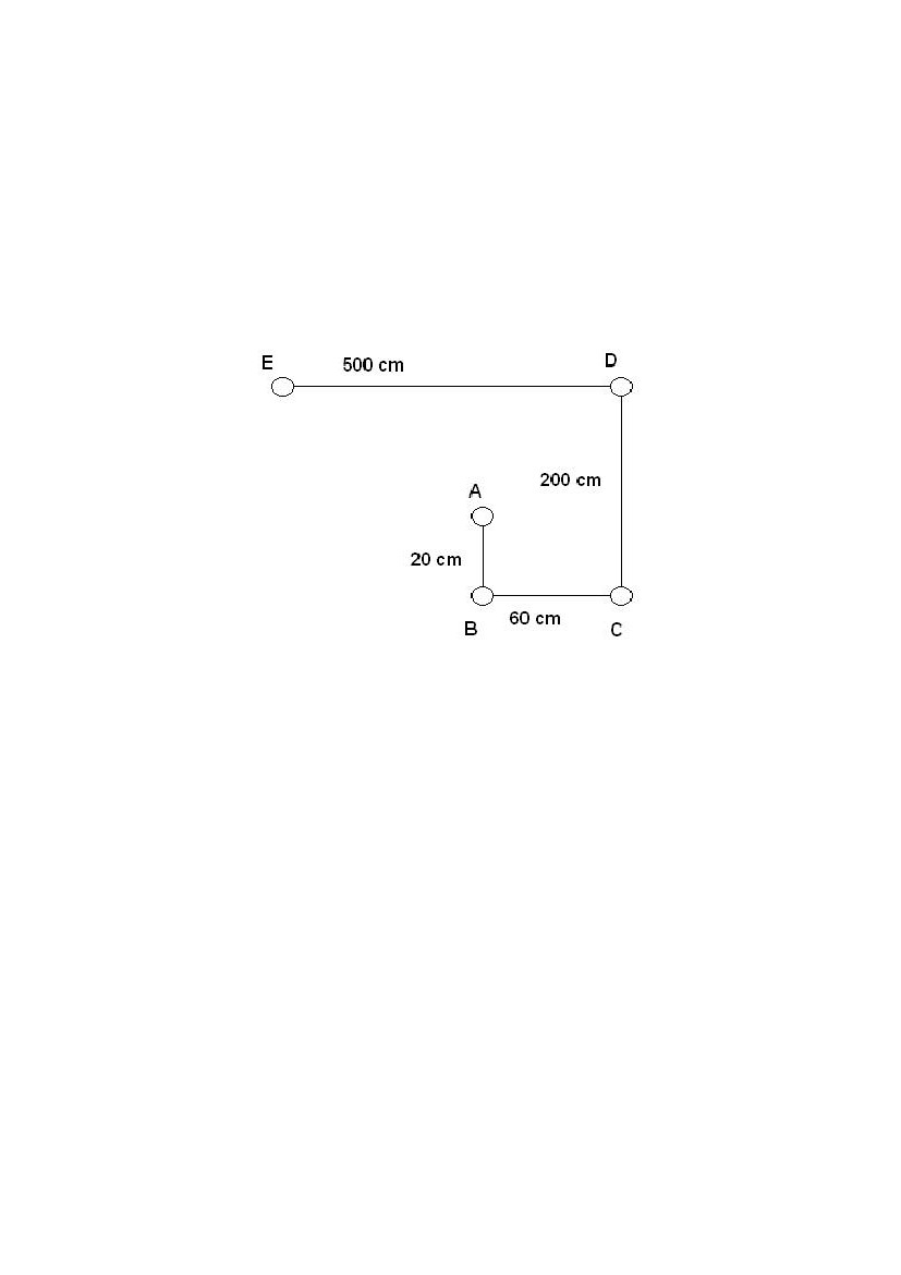
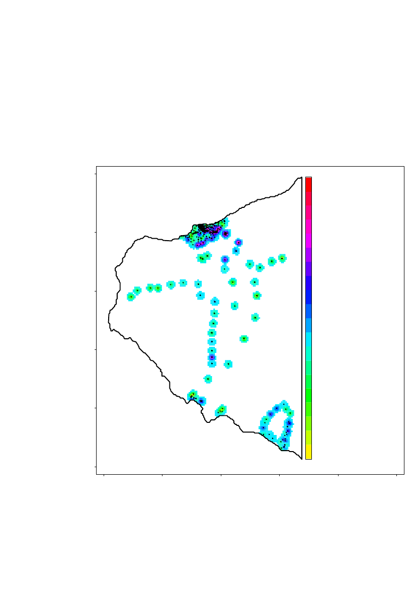
1 Geographic location of the measurementsThe geographic location is Thule, north-west Greenland. The gamma radiation levelof americium-241 (Bq/m2) is measured in the laboratory on soil samples and by aportable spectrometer on site. A total of 878 measurements were taken on 614locations. On some locations several measurements (up to 5 per location) were takento explore small scale variability. The coordinates on these locations were shiftedaccording to Figure 1. The first data point is kept; the second is shifted 20cm to theSouth, the third is shifted 60 cm East from the second point, the fourth 2 m north ofthe third and finally the fifth is shifted 5m west of the fourth (Figure 1).
Figure 1 Shift pattern for data points at coincident locations
6
Risø-R-1791(EN)
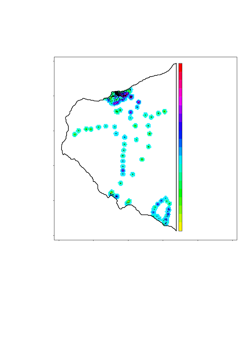
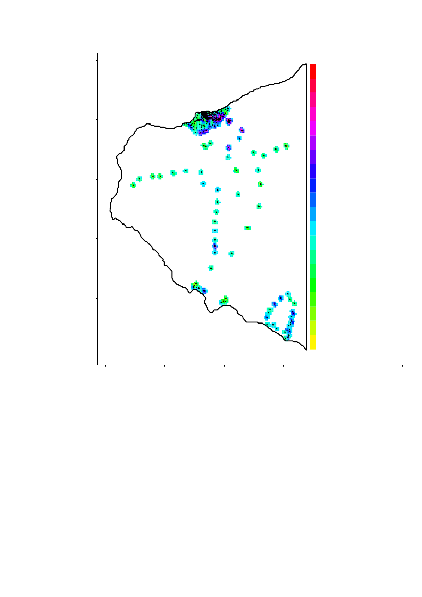
Coastline data was downloaded from (http://rimmer.ngdc.noaa.gov/) with a1:250.000 resolution (Figure 2).
76.8076.7576.7076.6576.60Latitude�N
Measurement locationsCoastline
76.5576.5076.4576.4076.3576.3076.2576.20-70.25 -70.00 -69.75 -69.50 -69.25 -69.00 -68.75 -68.50 -68.25 -68.00 -67.75Longitude�Ε
Figure 2 Coastline and location of measurements (Longitude,Latitude)
To be able to work and do spatial statistics with the data the coordinates weretransformed to metric coordinates. Thule is located in UTM-zone 19. The UTMcoordinates are shown in Figure 3.
8.521.2008.516.1008.511.0008.505.900UTM North zone 19
Measurement locationsCoastline
8.500.8008.495.7008.490.6008.485.5008.480.4008.475.3008.470.2008.465.1008.460.00010 km
465.000478.000491.000504.000517.000530.000471.500484.500497.500510.500523.500UTM East zone 19
Figure 3 Coastline and location of measurements (UTM-zone 19)
Risø-R-1791(EN)
7
The data are divided into different regions and analysed separately because theregions assumed to be independent, in the sense that the level of americium-241 isindependent from region to region (except region 2 being a subset of region 1). Theregions are shown in Figure 4.
Region 38.521.2008.516.1008.511.0008.505.900
Region 1Region 2Measurement locationsCoastline
Region 4
UTM North zone 19
8.500.8008.495.7008.490.6008.485.5008.480.4008.475.3008.470.2008.465.1008.460.00010 km
Region 6
Region 5465.000478.000491.000504.000517.000530.000471.500484.500497.500510.500523.500UTM East zone 19
Figure 4 Split in different geographic regions
Detailed spatial statistical analysis is performed for region the area around and southof Narsaarsuk including Grønnedal (region 1), for the area around Narsaarsuk(region 2) and also for a sub-region of approximately 1x1 km of Region 2.In the following regions only summary statistics is provided because data is to sparseto do spatial statistics:Region 3, the area around MoriusaqRegion 4, Saunders ØRegion 5, Wolstenholme ØRegion 6, the area near the Thule airbase
8
Risø-R-1791(EN)
2 Statistical methodsThe data is analysed using the package geoR (http://www.leg.ufpr.br/geoR) thatprovides functions for geostatistical data analysis using the software R (http://www.r-project.org/).Furthermore the packages splancs and maptools wereused for calculating neighbourhood distances and importing ESRI-Shapefiles for thealtitude data in region 1. Furthermore code was developed, to do simulations of thepredicted surface and calculate the total level of Americium and Plutonium alongwith 95% confidence intervals.The basic idea in spatial statistics is that data points close in space are morecorrelated than data points further apart. The geographic variation/correlationstructure is often described by a variogram, parameterised bynugget, sillandrange.Nuggetis the variation between samples taken at coincident or very close locations;sillis the variance between points at a distance where they are no longer correlated(that distance is denotedrange).The parameters are illustrated in Figure 5. In thesoftware used thepartial sill=sill – nuggetis estimated. Thesillis then found byaddingnuggetandpartial sill.
Sill
Variance
DataFit
NuggetDistance between observationsFigure 5 Theoretical variogram
Range
2.1
Likelihood based parameter estimation
The correlation structure is estimated using model based spatial statistics. The mainfunction estimate the parameters of the Gaussian random field model, specified as:
Y(x) = mu(x) + S(x) + ewhere•••
xdefines a spatial location.Yis the variable observed (log10(241Am)).mu(x) = X %*% betais the mean component of the model (a mean or atrend).
Risø-R-1791(EN)
9
•
S(x)is a stationary Gaussian process with variancesigma^2(partial sill) anda correlation functionrho(h)parameterised byphi(the range parameter) as:rho(h) = 1 - 1.5 * (h/phi) + 0.5(h/phi)^3 if h < phi , 0 otherwise(h is thedistance between point pairs) and the anisotropy parametersphi_Randphi_A(anisotropy ratio and angle, respectively) .eis the error term with variance parametertau^2(nugget variance).
•
A parameterλallows for the Box-Cox transformation of the response variableY.If used (i.e. ifλ≠1) Y(x)above is replaced byg(Y(x))such thatg(Y(x)) = ((Yλ(x)) - 1)/λ.Two particular cases areλ= 1which indicates no transformation andλ= 0indicating the log-transformation.The mean component of the model is assumed to be a constantmu(x) = beta0or afirst order polynomial on the coordinatesmu(x) = beta0+ beta1•x + beta2•y.The geometric anisotropy is described by the Anisotropy anglephi_A,defined hereas the azimuth angle of the direction with greater spatial continuity, i.e. the anglebetween the y-axis and the direction with the maximum range. Anisotropy ratiophi_R,defined here as the ratio between the ranges of the directions with greater andsmaller continuity, i.e. the ratio between maximum and minimum ranges. Therefore,its value is always greater or equal to one.For all datasets, a full model with all parameters (including trend and anisotropy) areestimated simultaneously in the maximum likelihood estimation. To avoidoverfitting, the model is reduced based on Akaike’s Information CriteriaAICandBayesian Information Criteria,BIC.Akaike Information Criteria is defined as AIC=-2 ln(L) + 2 p where L is themaximised likelihood and p is the number of parameters in the model.Bayesian Information Criteria is defined as BIC=-2ln(L) + p log(n), where n is thenumber of data, L is the maximised likelihood and p is the number of parameters inthe model.AIC is aimed at finding the best approximating model to the unknown true datagenerating process. AIC tries to select the model that most adequately describes anunknown, high dimensional reality. This means that reality is never in the set ofcandidate models that are being considered. BIC is designed to find the mostprobable model given the data BIC tries to find the true model among the set ofcandidates. Numerically BIC differs from AIC only in the second term which nowdepends on sample size n.An individual AIC value and individual BIC value is meaningless, but differences inAIC values and BIC values are meaningful. For both information criteria a smallervalue is better.There is no consensus about which criteria is the optimal to use. When comparingthe Bayesian Information Criteria and the Akaike’s Information Criteria, the penaltyfor additional parameters is higher in BIC than AIC. Here, both criteria are reported.In general the two criteria agree on the selected model and in case of disagreementboth models is reported and discussed and one is selected.
10
Risø-R-1791(EN)
2.2
Validation
The estimated model/correlation structure is validated by looking at theresiduals of the model. The residuals should be normal distributed and thereshould be no spatial correlation. Furthermore the profile-likelihood of each ofthe spatial parameters is presented.2.3Spatial prediction
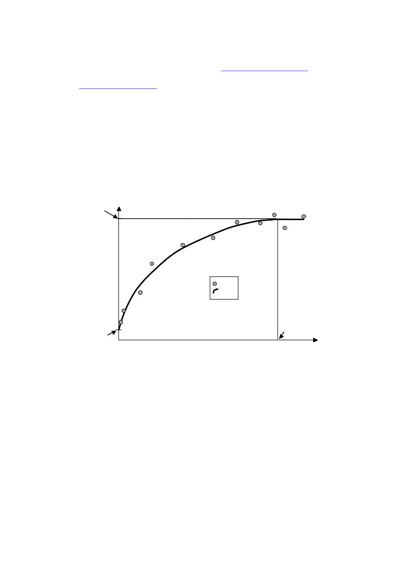
Spatial prediction onto a grid can be done once the spatial correlation structure isestimated. Only grid points on land are included. To estimate the concentration on alocation that has not been sampled a weighted average of all points within therangeis calculated (Figure 6). The weight allocated to each point depends on the distanceand the estimated correlation structure.25000
Rang20000Ykoord00
5000
10000
15000
5000
10000Xkoord
15000
Figure 6 Illustration of spatial prediction on a grid. The two grey locations (outside therange)have no weight in the prediction.
If significant anisotropy or trend is present these parameters are also included in theweighting and prediction.
2.4
Uncertainty of spatial prediction
Confidence intervals for the estimated spatial parameters are calculated as profile-likelihood intervals, so the are not necessary symmetric. The 90% and 95%confidence intervals are calculated as the value of the maximised log-likelihood -0.5×χ20.90(1) or 0.5×χ20.95(1), respectively. The intersections of the profile likelihoodcurves are shown in the profile likelihood plots for the spatial parameters: nugget,partial sill and range.
Risø-R-1791(EN)
11
The amount and uncertainty of241Am(Bqm-2) at each grid point (the predictionlocations) is based on the selected model. Based on the model a predictedconcentration and a prediction variance is calculated. The error is assumed normaldistributed so standard statistical uncertainty measures can be calculated for thepredicted values at each grid point. The following 3 is presented•The relative standard deviation•The upper 95% confidence limit•The probability of exceeding a threshold (log10(241Am)=2 andlog10(241Am)=3)
2.5
Prediction of the total amont of Plutonium239,240Pu
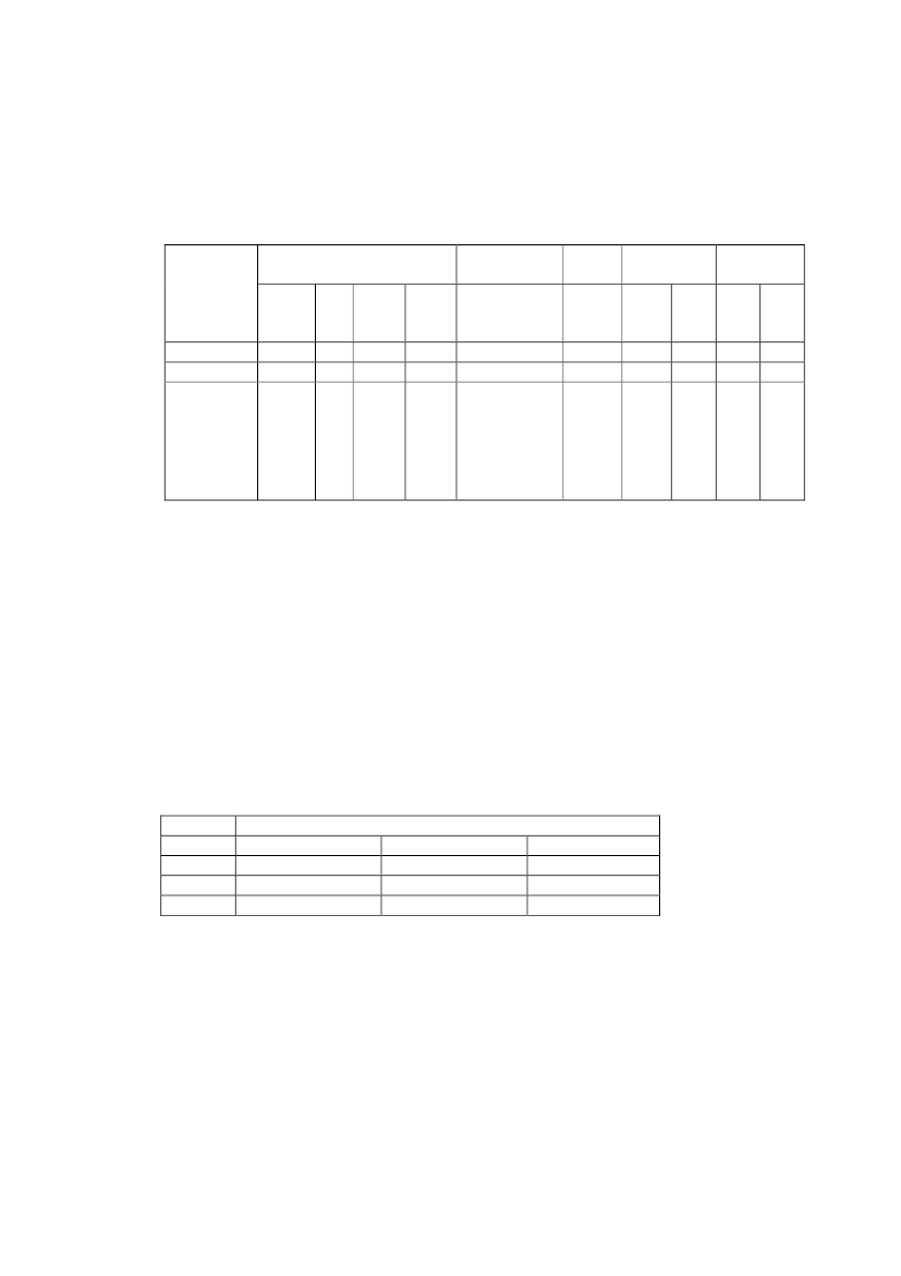
Based on the predicted contamination levels of241Am it is possible to predict thecontamination level of Plutonium (239,240Pu). The relationship between241Am and239,240Pu is shown in the table belowLevel of241
Am
<50Bqm
-2
>=50Bqm-2and<=1kBqm-24×241Am
>1kBqm-26×241Am
Calculated level of239,240Pu
3×241Am
Table 1 Calculation of the Plutonium level based on the Americium level
Each grid point (the prediction locations) represents a square.y
For each grid point a predicted level and a predictedvariance is calculated. The level of americium-241 ingrid squareiis calculated as the product of the area ofthei’thsquare (Ai=x•y) and the predicted level ofAmiin thei’thgrid point: Ai×Ami. The sum over theentire area is equivalent to the sum over the entire grid∑(Ai×Ami). Since all grid points represents an area ofthe same size the sum can be calculated as A×∑Ami.
X
The level239,240Pu is calculated by multiplying thepredicted level of Amiin thei’thgrid point by the factors from the table above andthen calculating the sum of239,240Pu for the entire area as described for241Am.Prediction of the level of241Am and239,240Pu will only be performed in grid pointslocated within the estimatedrangeform the nearest observed location. This approachhas been chosen to avoid a bias in the prediction. In the spatial statistical modelapplied, grid points with a larger distance to the nearest observed location than theestimatedrangewill be set to the mean component of the model. This is based on theassumption that the best guess of the level in such a location is the mean. However,if sampling in the area of interest has been targeted at specific locations where thelevel is high, this will results in an upwards biased predicted level in the locationsoutside the estimatedrange.Leaving out the prediction in some remote grid pointsdoes not imply that the level is 0, just that there is no information to base theprediction on.The uncertainty of the total predicted level of241Am and239,240Pu is estimated bysimulation. Based on the estimated spatial model a predicted level and a predictedvariance are calculated at each grid point. A random sample from each gridpoint isdrawn from a N(�i,σi2), where i denote the ithgrid point. The total level of241Am
12
Risø-R-1791(EN)
and239,240Pu is then calculated as described above. This is repeated 10000 times andthe 2.5% and 97.5% quantile is used as an empirical 95% confidence interval for thepredicted level of241Am and239,240Pu.The simulations are performed for all three models: The basic, the trend model andthe model including anisotropy.For the selected model in region 2 and the sub-region 2 further simulations areperformed that also take into account the uncertainty of the estimated spatialparameters. This is done by sampling from the 95% confidence intervals of thenugget, partial sill and range. For each sample, the predicted level of americium andthe related prediction variance is calculated and simulation is performed. Theconfidence intervals for the total level of241Am and239,240Pu will be wider than theconfidence intervals based on the simulations from the selected model.The following chapters will present the spatial statistical analysis, divided into thedescribed regions
Risø-R-1791(EN)
13
3 Analysis of data in Region 1This section describes the analysis of data in region 1 (see Figure 4). All spatialstatistics is performed on log10transformed data.
3.1
Geographical location
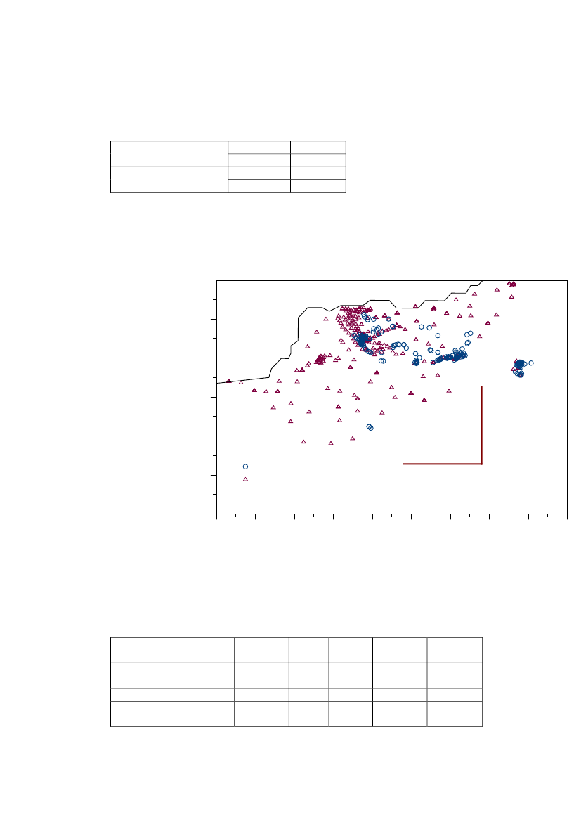
In region 1 a total of 805 measurements were taken on 561 locations, 625 soilsamples and 180 CAP measurements. The locations are shown in Figure 7
8.487.0008.485.0008.483.0008.481.000
CAPSoilCoastline
UTM North zone 19
8.479.0008.477.0008.475.0008.473.0008.471.0008.469.0008.467.000483.000487.000491.000495.000499.000503.000485.000489.000493.000497.000501.000UTM East zone 191 km
Figure 7 Data points in Region 1.
The locations in region 1 is bound by the following coordinatesEast (UTM zone 19)North (UTM zone 19)MaximumMinimumMaximumMinimum50000048300084900008465000
The minimum point (483000, 8465000) is subtracted from the coordinates in thespatial statistical presentation.
14
Risø-R-1791(EN)
3.2
Descriptive statistics75%quantile7.3×1033.97497Maximum2.8×1055.420308
A summary of the measurement is shown inTable 2.Minimum25%Mean MedianRegion 1quantile241-Am (Bqm1297.0×1032.1×1022)Log10(241Am)0.04*1.42.62.3Distances0.1674746431741(m)Table 2 Summary statistics, region 1
*0.1 was added to the241Am concentrations to obtain numerical stability
A summary plot of the data in section 1 is shown in Figure 8
Risø-R-1791(EN)
15
25
20000
Y Coord10000 15000
5000
0
0
5000
10000X Coord
15000
20000
00
5000
Y Coord10000 15000
20000
25
1
2
3data
4
5
5
4
2
1
0
5000
10000 15000 20000X Coord
0.000
0
0.10
Density0.20
data3
0.30
1
2
3data
4
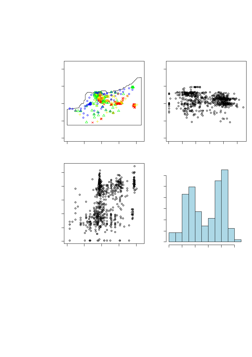
5
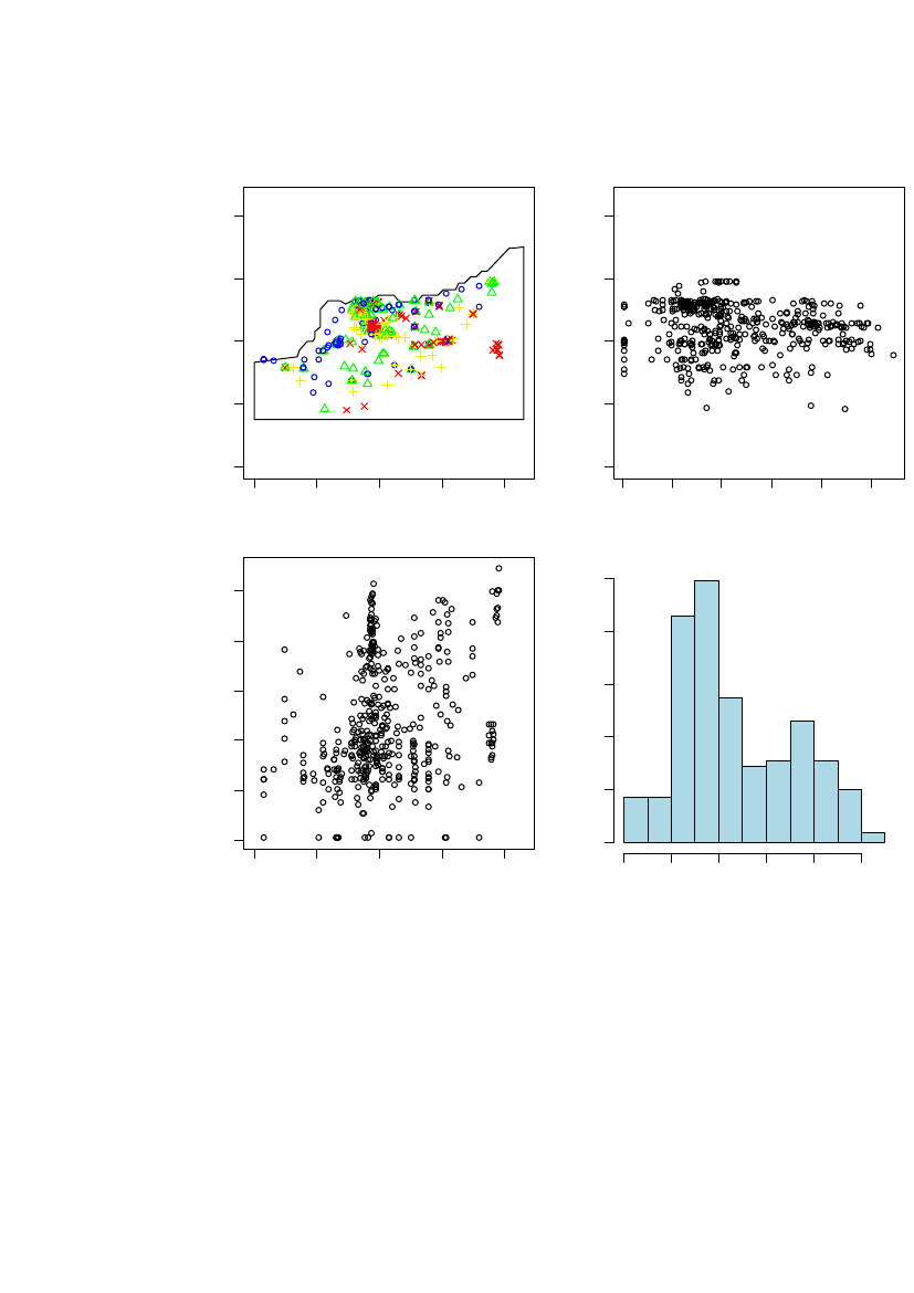
Figure 8 Summary plot of the log10(241Am) data in region 1. Upper left: Blue circle is the0-25% quantiles, green triangle is the 25-50% quantiles, yellow plus is the 50-75%quantiles and red cross is the 75-100% quantiles.
In Figure 8 it can be seen that high concentrations also exist outside the coastal area.The histogram shows a bi-modular distribution. The bi-modal data distribution mightreflect the sampling strategy, where the intension was to sample inside as well asoutside hot-spot areas. The bi-modal distribution does not affect the validity of aspatial statistical analysis.
3.3
Spatial correlation
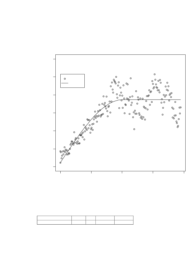
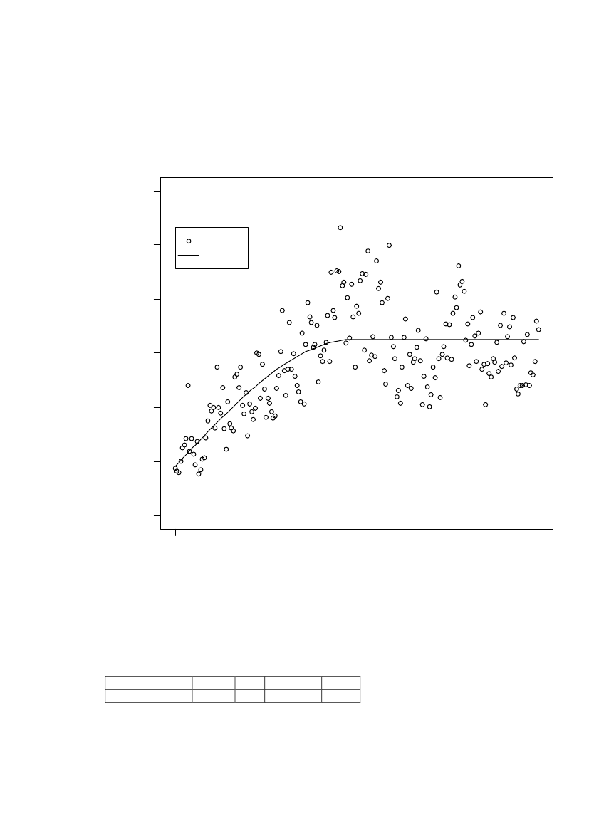
Before doing the maximum likelihood estimation an empirical variogram iscalculated. The calculated values and the fitted spherical variogram function isshown in Figure 9
16
Risø-R-1791(EN)
2.5
ValuesFit2.0Variance0.000.51.01.5
200
400
600Distance
800
1000
Figure 9 Variogram for log10(241Am) in Region 1. Distances are divided with bins ofapproximately 5 m.
Risø-R-1791(EN)
17
A very clear spatial correlation is seen. The parameters in the fitted sphericalvariogram function is shown in Table 3Variogram parameter Nugget Sill Partial Sill Range (m)Estimated value0.131.811.69391Table 3 Parameter values from nonlinear weighted regression of the variogram, region1.
So, preliminary it is assumed that data is correlated within a range of approximately400 m.
3.4
ML-estimation and prediction of contamination level
The spatial maximum likelihood (ML) estimation of the three models resulted in thecorrelation structure shown in Table 4ModelBox-coxTrendtransformationNugget Sill Partial Range LambdaBeta0,Sill(m)BetaX,BetaY0.4371.44 1.013800.8760.8991,38 0.9651,40 0.9652503740.8790.875Spatial parametersInformationcriteriaAngle Ratio AIC BICAnisotropy
Basicmodel+Anisotropy 0.412+trend0.437
2171 21941.982166 21992169 2207
0.9792.59-0.5568.7×10-5
4.0×10⁻⁵
Table 4 Parameter values from the maximum likelihood estimation in region 1.
Based on the AIC a model with anisotropy is the most optimal (smallest AIC). Basedon the BIC the basic model without trend or anisotropy is optimal (smallest BIC).The two model selection criteria disagree.In region 1 large areas are sparsely sampled, therefore it is decided to use the basicmodel without an overall spatial trend and without anisotropy (marked in bold in theTable 4 above).Based on the ML-estimation data is correlated within a distance of 380 m. Thecorrelation is not depending on direction. This implies that locations further awaythan 380 m from a measurement location can not be predicted based on themeasurements. The partial sill is approximately 2 times higher than the nugget.The 90% and 95% confidence intervals for the spatial parameters are shown inML-estimate and 95% profile likelihood confidence intervalsNuggetPartial sillRangeEstimate0.441.038090% CI[0.35;0.52][0.98;1.0][340;>1000]95%CI[0.37;0.54][0.99;1.0][320;>1000]
18
Risø-R-1791(EN)
Table 5 Maximum likelihood estimates and 90% and 95% profile likelihood confidenceintervals for the spatial parameters in region 1
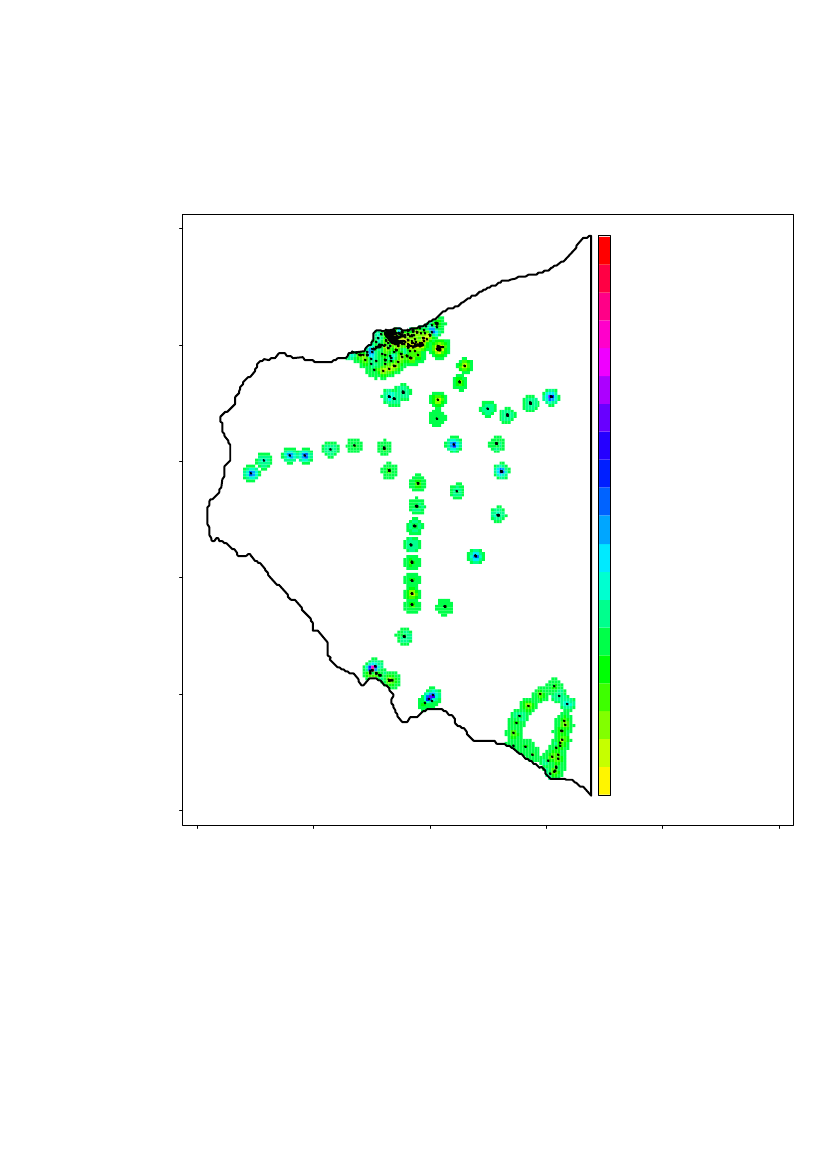
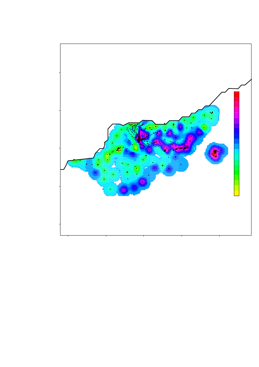
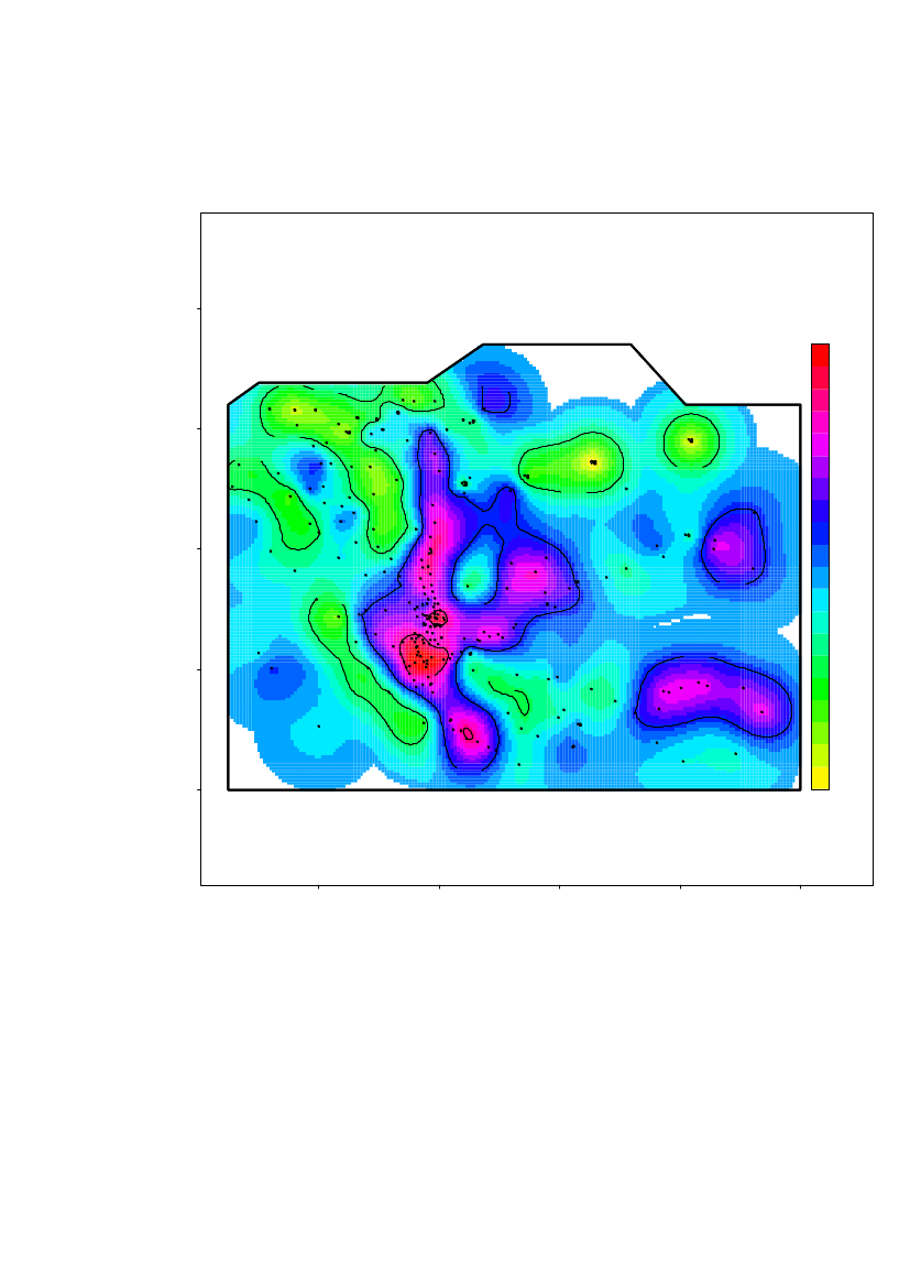
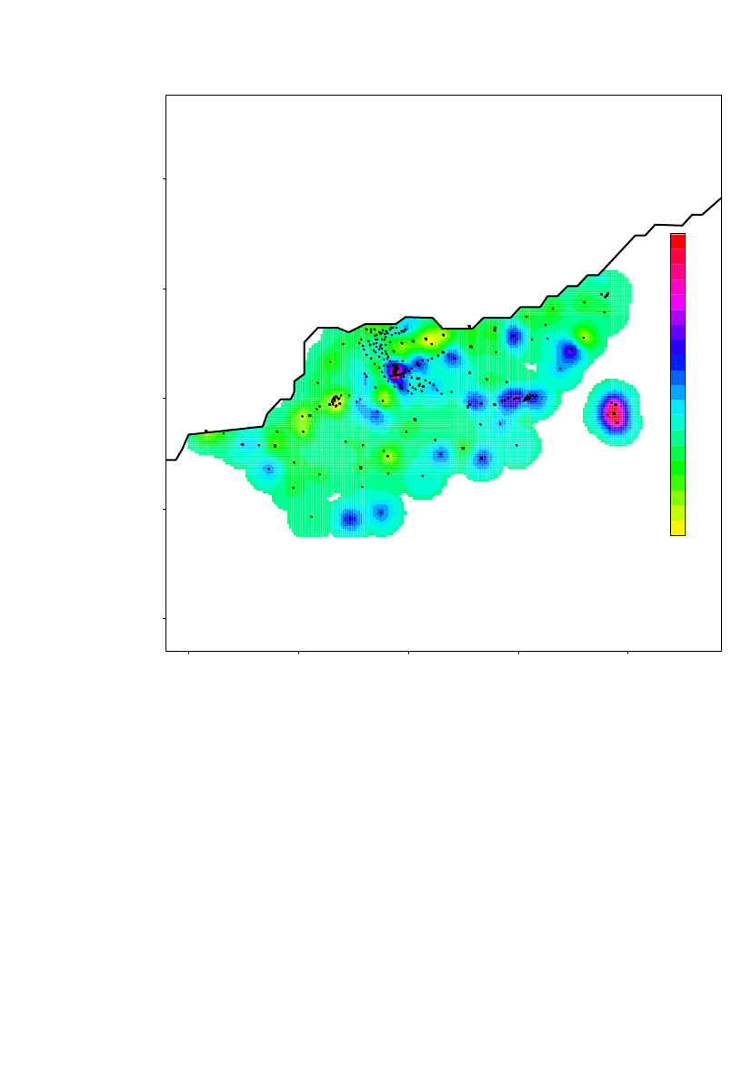
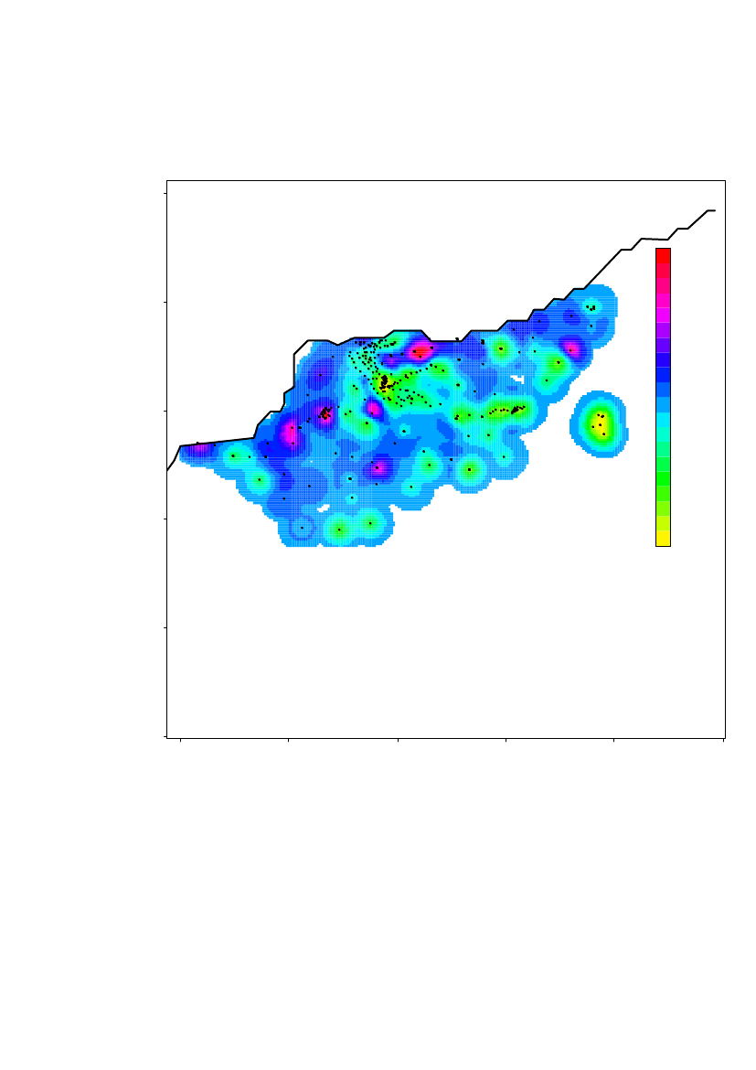
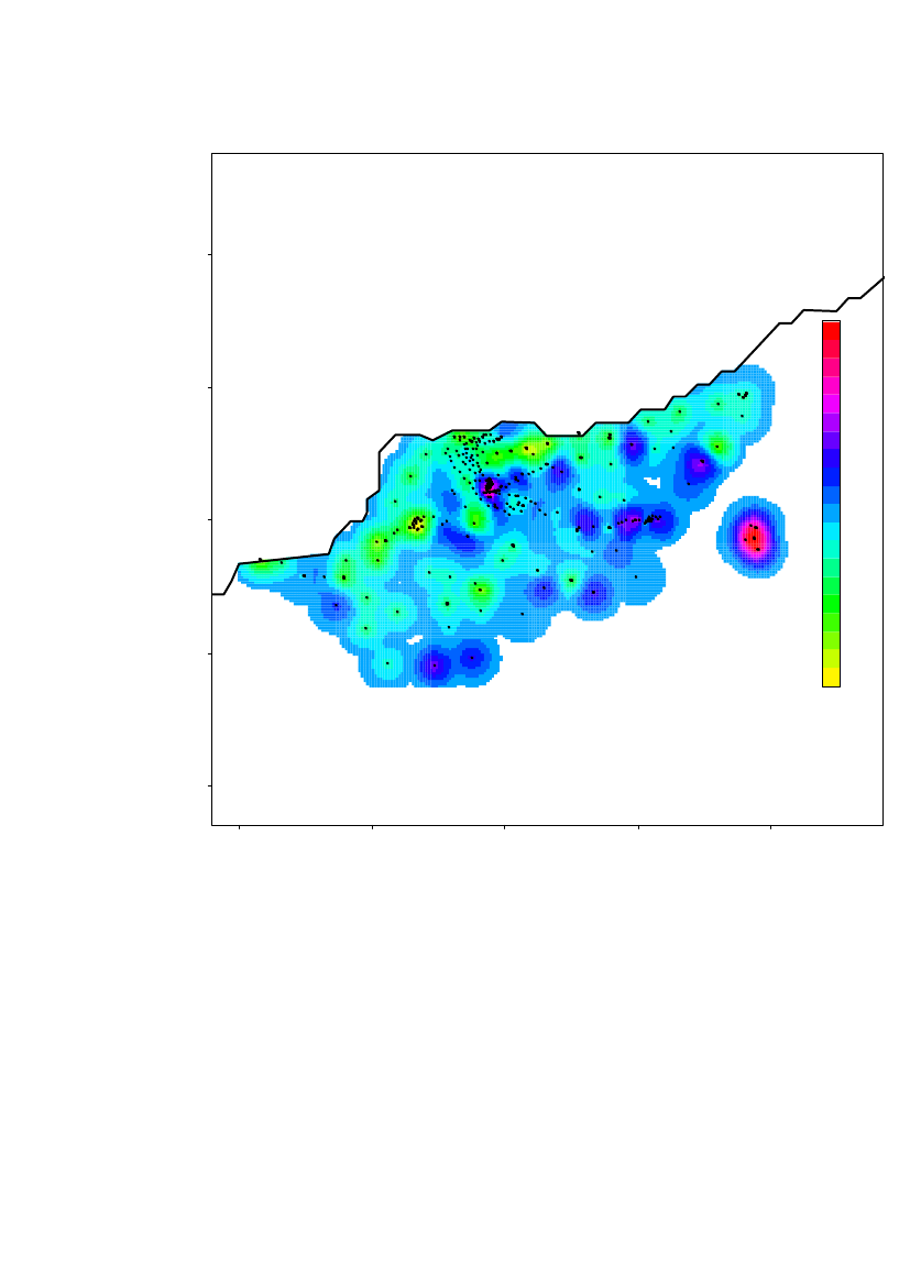
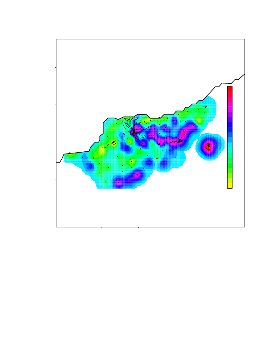
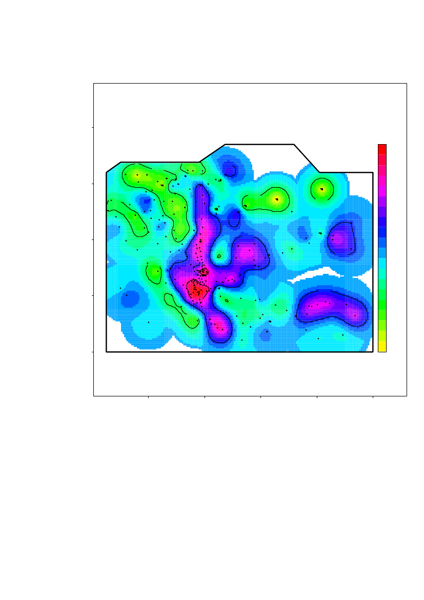
The spatial prediction on a 100m×100m grid of the log10(Am) concentrations inregion 1 is shown in Figure 10. Locations further than 380 m from a measurementlocation are not predicted. The altitude is overlaid the predicted concentrationsshown by height curves.Based on the estimated range, it is evident that further sampling is needed to estimatethe contamination level in the entire area.
25000
The highest contamination level is located in the area around Narsaarsuk.
420000Latitude (m)15000
3
10000
2
5000
1
00
5000
10000
15000Longitude (m)
20000
25000
Risø-R-1791(EN)
19
3.5
Validation of spatial maximum likelihood estimation
Standard normal quantile-1012
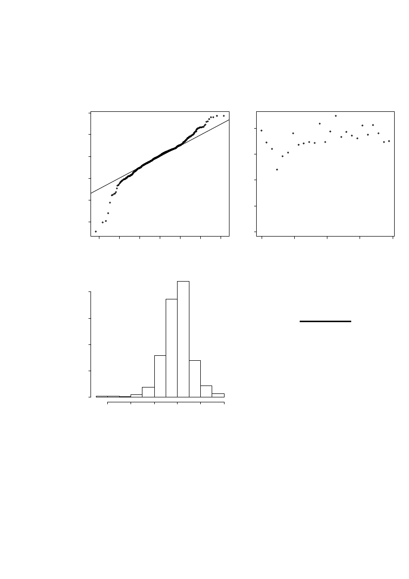
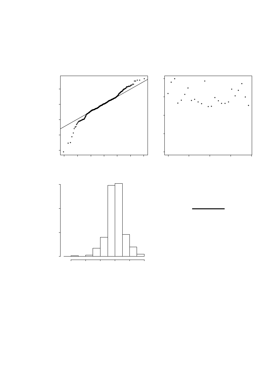
In Figure 11 the residuals from the maximum likelihood estimation is evaluated. TheQQ-plot, Histogram and the Box-Whisker plot show approximately normaldistributed data. The variogram show a small spatial dependency with data pointsvery close having slightly less variance. However, with an estimated partial sill of 1the small correlation in the residuals is not considered of major importance.0.4
QQ-plot
Variogram
-3
-2
-3
-2
-1
01Residuals
2
3
0.00
0.1
Variance0.20.3
200
400600distance (m)
800
0
50
Frequency100 150 200 250 300
Histogram
-3
-2
-1x3
0
1
2
20
Risø-R-1791(EN)
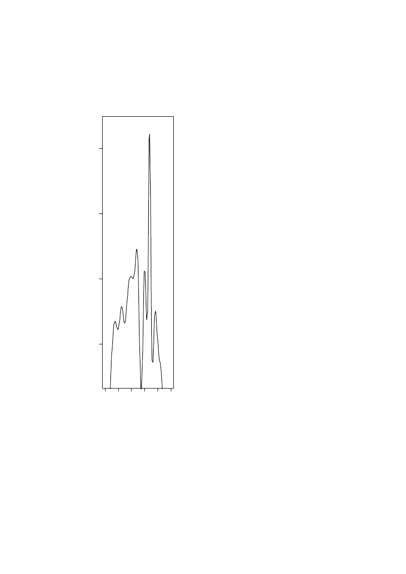
Profile-likelihood curvesIn Figure 12 the profile likelihood is shown for the final basic model of Region 1.Only the nugget has a nice bell-shaped curve. The dotted horizontal lines indicateapproximate 90% and 95% confidence intervals for each parameter.
profile log-likelihood
-10900.8
-1088
-1086
-1084
-1082
-1080
0.9
1.02
1.1
1.2
Risø-R-1791(EN)
21
3.6
Uncertainty of predicted contamination level
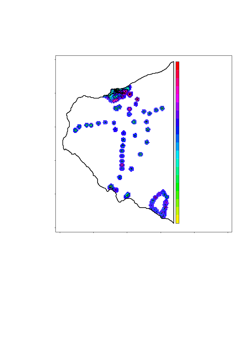
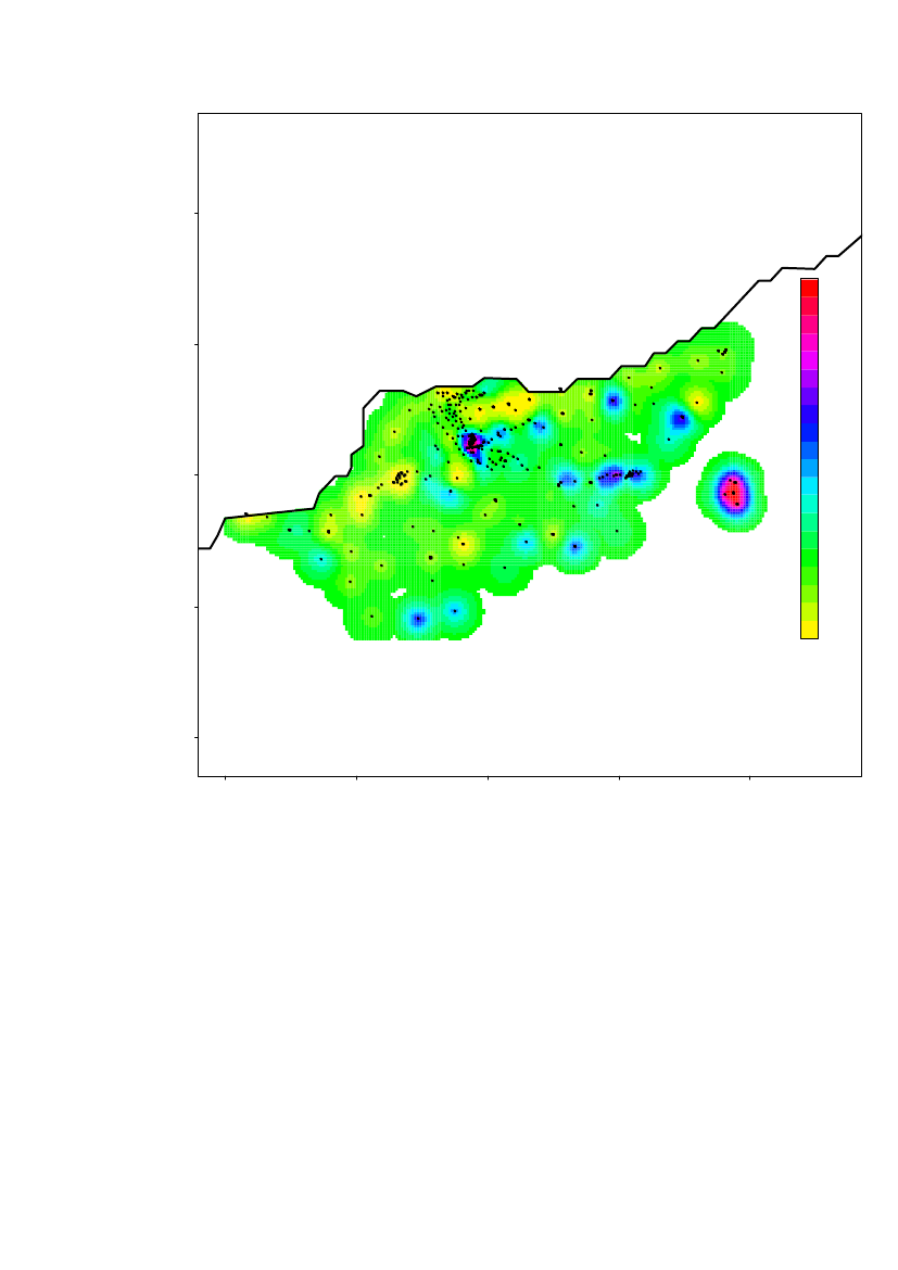
The relative standard error (standard error/predicted value) of the predictedconcentrations are shown in Figure 13. The relative error is in general small in themore densely sampled areas. It does of course also depend on the local variation.
25000
1.7200001.61.51.4Latitude (m)10000150001.31.21.110.90.80.750000.60.50.40.3
00
5000
10000
15000Longitude (m)
20000
25000
22
Risø-R-1791(EN)
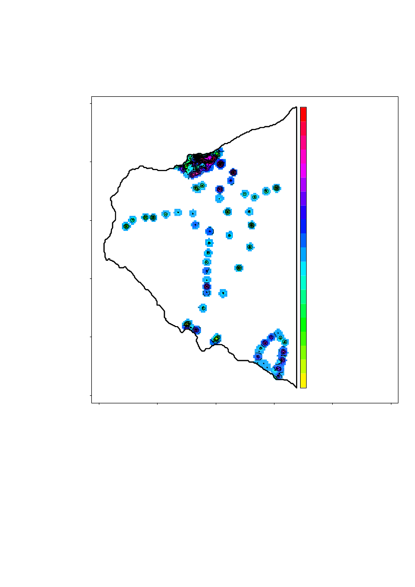
Based on the standard error of each predicted value the upper 95% confidence limitfor the predicted values is shown in Figure 14. Notice that it is a point-wise 95%confidence interval, so it is not a 95% confidence interval for the surface as such. Itcan however be used to evaluate the upper limit for each grid-point
25000
6200004
4
5Latitude (m)15000
4
10000
35000
4
2
00
5000
10000
15000Longitude (m)
20000
25000
Risø-R-1791(EN)
23
Based on normal probability assumptions the probability that the concentrationexceeds a certain threshold can be calculated. In Figure 15 and Figure 16 theprobability of the log10concentration exceeding 2 and 3 respectively is shown.
25000
0.95200000.90 .40 .30.5
0 .5
0.850.6
0.50 .70 .6
0.80.750.70.650.60.550.50.450.40.350.30.25
Latitude (m)1000015000
0 .5
5000
0 .5
0.20 .4
0.150.10.050 .5
00
5000
10000
15000Longitude (m)
20000
25000
24
Risø-R-1791(EN)
25000
0.9200000.850.2
0 .2
0.80.3
0.1
0.20 .4
0.750.70.650.60.550.50.450.40.350.30.25
0.3
5000
10000
Latitude (m)15000
0 .2
0.20.2
0.20 .2
0.150.10.05
00
5000
10000
15000Longitude (m)
20000
25000
Risø-R-1791(EN)
25
3.7
Conclusion region 1
A clear spatial correlation structure is present in region 1. The basic spatial modelwith nugget, partial sill and range as spatial parameters was selected.Data are correlated up to a distance of approximately 380m (estimatedrange).Thepartial sill was estimated to be 1 and the nugget approximately 0.5, so the partial sillis 2 times the nugget.Due to the size of the area and the sampling performed, large areas are further than380m away from the nearest observation. This means that the information in thesampled points is of no use in these areas, resulting in the average concentrationbeing the best guess. This most likely doesn’t reflect reality so interpretation in theseareas should not be done based on the presented data. Further sampling is needed toconclude anything in these areas.In region 1 the maximum observed level of241Am was 2.8×10⁵Bqm-2. Most highlevels were observed near Narsaarsuk. This area was also sampled most intensively.However, in Grønnedal the maximum observed level of241Am was 1.9×10⁴Bqm-2.Based on the topography of the area and the location of the hot-spots a hypothesiscould be wind, snow and water transport particles to pools where the level thereforeincrease.The area is so sparse sampled that it is of no use to try to predict the overall amountof241Am and239,240Pu. This is only done for region 2.
26
Risø-R-1791(EN)
4 Analysis of data in Region 2This section describes the analysis of data in region 2 (see Figure 4)
4.1
Geographical location
The locations in region 2 is bound by the following coordinatesEast (UTM zone 19)Maximum494000Minimum489500North (UTM zone 19)Maximum8486000Minimum8483000The minimum point (489500, 8483000) is subtracted from the coordinates in thespatial statistical presentation. A total of 615 measurements were taken on 439locations, 435 soil samples and 180 CAP measurements. The location is shown inFigure 17
8.486.000
8.485.500
UTM North zone 19
8.485.000
8.484.5001 km
8.484.000CAPSoilCoastline
8.483.500
8.483.000489.500 490.000 490.500 491.000 491.500 492.000 492.500 493.000 493.500 494.000UTM East zone 19
Figure 17 Location of sampling points in region 2
4.2
Descriptive statistics75%quantile1.0×1044.01370Maximum2.8×1055.43890
A summary of the measurement is shown in Table 6Minimum25%Mean Medianquantile241-Am (Bqm1.1488.11.2×1032)×103Log10(241Am)0.04*1.72.83.1Distances0.16435987888(m)
Risø-R-1791(EN)
27
Table 6 Summary statistics, region 2
*0.1 was added to the concentrations to obtain numerical stabilityAll spatial statistics is performed on log10transformed data. A summary plot isshown in Figure 18400040000100020003000Longitude (m)4000001000Latitude (m)20003000
0
1000
Latitude (m)20003000
1
2
34Log10(Am)
5
2
1
0
0
1000
20003000Longitude (m)
4000
00
20
40
Frekvens6080100
Log10(Am)34
120
5
1
2
34Log10(Am)
5
Figure 18 Summary plot of the log10(241Am) data in region 2. In the upper left: Bluecircle is the 0-25% quantiles, green triangle is the 25-50% quantiles, yellow plus is the50-75% quantiles and red cross is the 75-100% quantiles.
From Figure 18 it can be seen that high concentrations exist throughout the area. Thehistogram shows a bi-modular distribution. The bi-modal data distribution mightreflect the sampling strategy, where the intension was to sample inside as well asoutside hot-spot areas. The bi-modal distribution does not affect the validity of aspatial statistical analysis.
28
Risø-R-1791(EN)
4.3
Spatial correlation
Before doing the maximum likelihood estimation a variogram is calculated. Thecalculated values and the fitted spherical variogram function is shown in Figure 19
2.5
3.0
ValuesFit2.0Variance0.000.51.01.5
200
400Distance
600
800
Figure 19 Variogram for log10(Am) in Region 2
A very clear spatial correlation is seen. The parameters in the fitted sphericalvariogram function is shown in Table 7Variogram parameter Nugget Sill Partial Sill Range (m)Estimated value0.111.87 1.75402Table 7 Parameter values from nonlinear weighted regression of the variogram, region2
Risø-R-1791(EN)
29
So, preliminary it is assumed that data is correlated within a range of approximately400 m
4.4
Prediction of contamination level
As for region 1 the basic model and more complex models were investigated; 1)Including a 1storder trend and/or 2) including anisotropy. The spatial maximumlikelihood estimation resulted in the correlation structure shown in Table 8.ModelSpatial parametersNugget Sill PartialSillBasic model 0.556 1.83 1.27+Anisotropy 0.548 2.80 2.25+trend0.556 1.49 0.938Box-coxTrend AnisotropytransformationRangeLambdaBeta0, Angle Ratio(m)BetaX,BetaY2801.071.455841.061.42 2.61 1.801981.081.707.6×10-4
InformationcriteriaAIC BIC
1645 16671641 16721628 1659
-9.0×10⁻⁴
Table 8 Parameter values from the maximum likelihood estimation in region 2.
Based on the AIC and BIC a model with a first order trend is the most optimal. Thetwo model selection criteria agree. Therefore it is decided to use the model with anoverall spatial trend.Based on the ML-estimation data is correlated within a distance of 198m. Thecorrelation is not depending on direction. This implies that locations further awaythan 198 m from a measurement location can not be predicted based on themeasurements. The partial sill is approximately 2 times higher than the nugget.The 90% and 95% profile likelihood confidence intervals for the spatial parameters(nugget, partial sill and range) of the selected model are shown in Table 9ML-estimate and 95% profile likelihood confidence intervalsNuggetPartial sillRangeEstimate0.560.9419890% CI[0.45;0.69][0.76;0.95][109;292]95%CI[0.44;0.72][0.64;1.0][103;302]Table 9 Maximum likelihood estimates and 90% and 95% profile likelihood confidenceintervals for the spatial parameters in region 2.
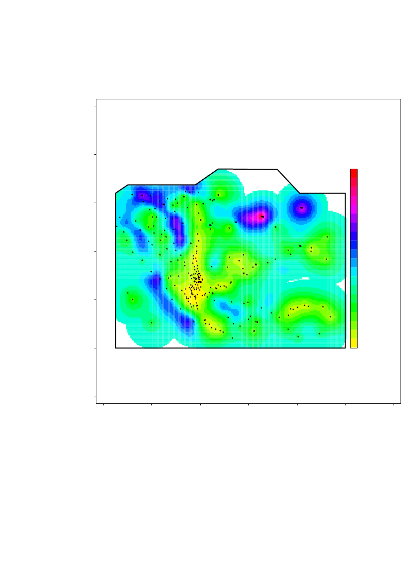
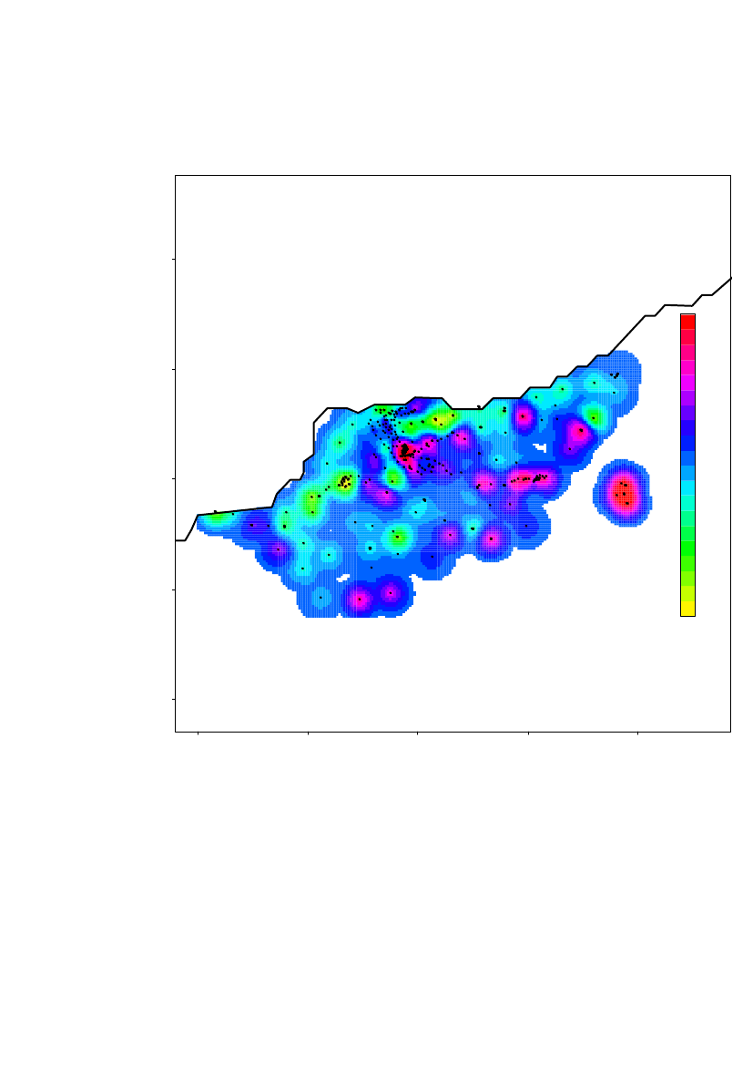
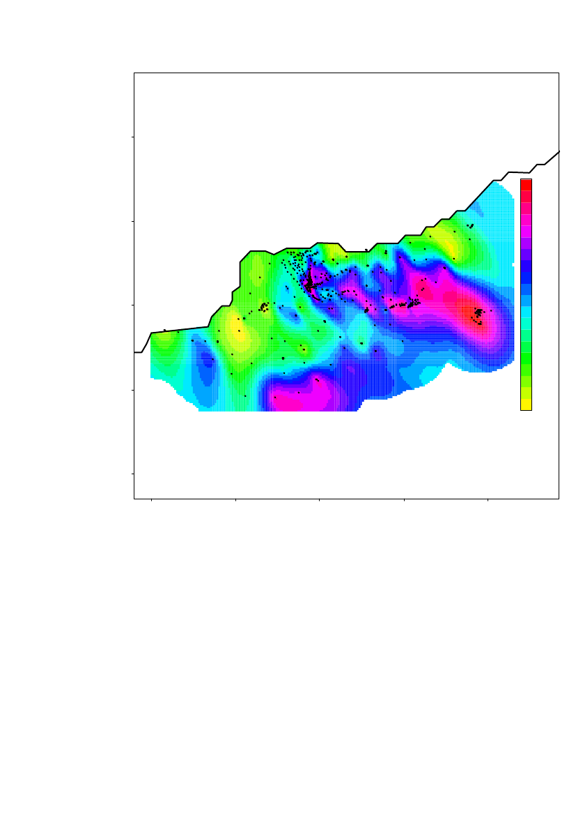
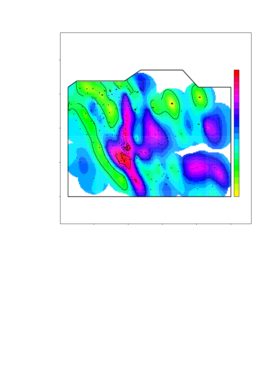
The spatial prediction on a 20m×20m grid of the log10(Am) concentrations in region2 is shown in Figure 20 with height curves overlaid. Locations further than 198 mfrom a measurement location is not predicted.The 1storder trend parameters (Beta0, BetaX and BetaY) show that the Americiumlevel increase in south-east direction
30
Risø-R-1791(EN)
Latitude (m)20003000
4000
4
3
21000
1
00
1000
2000
3000Longitude (m)
4000
Risø-R-1791(EN)
31
4.5
Validation of spatial maximum likelihood estimation
Standard normal quantile-1012
In Figure 21 the residuals from the maximum likelihood estimation is evaluated. TheQQ-plot, Histogram and the Box-Whisker plot show approximately normaldistributed data. The variogram show no spatial dependency.
QQ-plot0.4
Variogram
-2
-3
-3
-2
-1
10Residuals
2
3
0.0
0.1
Variance0.20.3
0
100
200300distance (m)
400
Histogram200050Frequency100150
-3
-2
-1x3
0
1
2
32
Risø-R-1791(EN)
Profile-likelihood curvesIn Figure 22 the profile likelihood is shown for the model with 1storder trend forregion 2. The dotted horizontal lines indicate approximate 90% and 95% confidenceintervals for each parameter.
profile log-likelihood
-808.50.6
-808.0
-807.5
-807.0
0.7
0.82
0.9
1.0
1.1
Risø-R-1791(EN)
33
4.6
Uncertainty of predicted contamination level
The relative standard error (standard error/predicted) of the predicted concentrationsare shown in Figure 23. The relative error is in general small in the more denselysampled areas. It does of course also depend on the local variation.4000
1.1300010.90.80.7
Latitude (m)
2000
0.60.50.4
1000
0.30.2
-10000
0
1000
2000
3000
4000
5000
Longitude (m)
34
Risø-R-1791(EN)
Based on normal probability assumptions the probability that the concentrationexceeds a certain threshold can be calculated. In Figure 24 and Figure 25 theprobability of the log10(241Am) concentration exceeding 3 and 2 respectively isshown.
4000
3000
0.950.90.850.80.750.70.650.60.550.50.450.40.350.30.250.20.150.10.05
Latitude (m)010002000
0
1000
2000
3000
4000
Longitude (m)
Risø-R-1791(EN)
35
4000
0.9530000.90.850.80.750.70.650.620000.550.50.450.40.350.30.2510000.20.150.1
Latitude (m)0
0
1000
2000
3000
4000
Longitude (m)
36
Risø-R-1791(EN)
4000
63000
2000
Latitude (m)
5
4
1000
3
00
1000
2000Longitude (m)
3000
4000
Risø-R-1791(EN)
37
4.7
Prediction of239,240Pu
Based on the predicted surface of log10(241Am) the level of241Am and239,240Pu iscalculated as described in section 2.5. The results for the three models are listed inthe Table 10, with the optimal model including trend in bold.ModelTotal Area withinArearange(km2) from nearestneighbour(km2)8.005.648.008.007.244.93241
Basicmodel+Aniso+ Trend
Proportion Total241AmTotal239,240PuofGBq (Bq×109) GBq (Bq×109)total area[95% CI][95% CI]withinrange71%87[63;143]518[377;856]91% 569[287;1476] 3410[1717;8854]61%45[36;65]270[212;387]239,240
Table 10 Predicted level offound by simulation.
Am and
Pu in region 2. Confidence intervals are
As can be seen in Table 10, the area where the level of241Am and239,240Pu ispredicted depends on the model or more specifically on the estimated range of themodel.The higher the estimated range the larger area is included. Furthermore,measurements with high levels have influence on a larger area in models with largerrange.For the optimal model 61% corresponding to 4.93 km2of the total 8.00km2wereincluded and the predicted total amount of241Am is 45 GBq (Bq×109). The predictedtotal amount of239,240Pu is 270 GBq (Bq×109).Based on simulations, the confidence intervals for the total level of241Am and239,240Pu is Table 11241
Simulations based on the estimated trendmodel.Simulations as above and in additionincluding uncertainty of spatial parameters
Am [95%CI](GBq)[36;65][ 24;82]241
239,240
Pu [95%CI](GBq)[212;387][140;490]
Table 11 Confidence intervals of the total level ofsimulation in region 2.
Am and
239,240
Pu, based on
38
Risø-R-1791(EN)
If locations with a distance to nearest measurement location larger than the estimatedrange is included in the prediction, the predicted total level of241Am and239,240Puincrease as described in the table belowTotal241AmTotal239,240PuTBq (Bq×1012) TBq (Bq×1012)Basic model132793+Aniso7664594+ Trend73442ModelTable 12 Predicted level of241Am and239,240Pu in region 2 including locations furtherthan the estimated range away from the nearest measurement location.
4.8
Conclusion region 2
A clear spatial correlation structure is present in region 2. Data are correlated up to adistance of approximately 200m (estimated range=198m). A south-east trend wasobserved. Due to the size of the area and the sampling performed, some areas arefurther than 200m away from the nearest observation. In these areas the averageconcentration is best guess. This most likely doesn’t reflect reality so interpretationin these areas should be done with care. The partial sill was estimated to be 1 and thenugget approximately 0.5, so the partial sill is 2 times the nugget.Further sampling is needed to make more precisely conclusion about theconcentrations in these areas.Under the optimal spatial model, within the area of prediction, the predicted totalamount of241Am is 45[95%CI: 36;65] GBq (Bq×109) and the predicted total amountof239,240Pu is 270[95%CI: 212;387] GBq (Bq×109).Including the uncertainty of the estimated spatial parameters the confidence intervalsgets wider, thus within the area of prediction, the predicted total amount of241Am is45[95%CI: 24;82] GBq (Bq×109) and the predicted total amount of239,240Pu is270[95%CI: 140;490] GBq (Bq×109).Based on the topography of the area and the location of the hot-spots a hypothesiscould be wind, snow and water transport particles to pools where the level thereforeincrease.
Risø-R-1791(EN)
39
5 Analysis of a sub-region of Region 2This section describes the analysis of data in a 1x1 km coastal sub-region of region 2
5.1
Geographical location
The locations in the sub-region is bound by the following coordinatesEast (UTM zone 19)Maximum492000Minimum491000North (UTM zone 19)Maximum8486000Minimum8485000The minimum point (491000, 8485000) is subtracted from the coordinates in thespatial statistical presentationA total of 312 measurements were taken on 215 locations, 225 soil samples and 87CAP measurements. The location is shown in Figure 27
Ykoord
0
200
400
600
200
400
600Xkoord
800
1000
Figure 27 Location of a sub-region of Region 2
5.2
Descriptive statistics
A summary of the measurement is shown in Table 13.
40
Risø-R-1791(EN)
MinimumAm (Bqm-2)Log10AmDistances(m)10.04*0.16
25%quantile671.8160
Mean
Median
7.4×1031.7×1032.93013.2302
75%quantile9.2×1034.0418
Maximum1.4×1055.1965
Table 13 Summary statistics sub- region 2.
*0.1 was added to the concentrations to obtain numerical stabilityAll spatial statistics is performed on log10transformed data. A summary plot isshown in Figure 28800800200400600800Longitude (m)100000200Latitude (m)400600
0
200
Latitude (m)400600
1
2
34Log10(Am)
5
5
Log10(Am)34
2
1
0
200
400
600800Longitude (m)
1000
00
10
20
Frekvens3040
50
60
1
2
34Log10(Am)
5
Figure 28 Summary plot of the log10(Am) data in sub-region 2. In the upper left: Bluecircle is the 0-25% quantiles, green triangle is the 25-50% quantiles, yellow plus is the50-75% quantiles and red cross is the 75-100% quantiles.
Risø-R-1791(EN)
41
In Figure 28 it can be seen that high concentrations is evenly spread, although thereseems be one area with higher concentrations. The histogram shows a bi-modulardistribution.
5.3
Spatial correlation
Before doing the maximum likelihood estimation a variogram is calculated. Thecalculated values and the fitted spherical variogram function is shown in Figure 29
4
ValuesFit
Variance
00
1
2
3
200
400Distance
600
800
1000
Figure 29 Variogram for log10(Am) in the sub-region of Region 2
A very clear spatial correlation is seen. The parameters in the fitted sphericalvariogram function is shown in Table 14Spatial parameter Nugget SillPartial Sill Range
42
Risø-R-1791(EN)
Estimated value
0.05
2.01 1.96
387m
Table 14 Parameter values from nonlinear weighted regression of the variogram, region2
So, preliminary it is assumed that data is correlated within a range of approximately400 m
5.4
Prediction of contamination level
As for region 1 and 2 the basic spatial model and more complex models wereinvestigated: 1) Including a 1storder trend and/or 2) including anisotropy, meaningthat the spatial correlation is independent on direction. The spatial maximumlikelihood estimation resulted in the correlation structure shown in Table 15ModelNugget SillRange Lambda Beta0, Angle Ratio AIC(m)BetaX,BetaY1.046 1081.1591.76018031.475 0.9615 90.51.1462.763 2.033 8011.401 0.8678 98.91.1482.0274798-8.2×10⁴
PartialSill
BIC
Basic model 0.5357+Anisotropy* 0.5131+trend0.5331
822827825
-1.8×10⁻³
Table 15 Maximum likelihood parameter estimates for spatial models, in sub-region 2
Based on the AIC a model with a first order trend is the most optimal. Based on theBIC the basic model without trend or anisotropy is optimal. The two model selectioncriteria disagree.In this sub-area of region 2 the variability is assumed to be local, no overall trend isassumed to exist. Therefore it is decided to use the model without an overall spatialtrend.Based on the ML-estimation data is correlated within a distance of approximately108 m. The correlation is not depending on direction. This implies that locationsfurther away than 108 m from a measurement location can not be predicted based onthe measurements. The partial sill is approximately 2 times higher than the nugget.The 90% and 95% profile likelihood confidence intervals for the spatial parameters(nugget, partial sill and range) of the selected model are shown in Table 16ML-estimate and 95% profile likelihood confidence intervalsNuggetPartial sillRangeEst0.541.0410890% CI[0.38;0.82][1.04;1.05][88;157]95%CI[0.36;0.85][1.04;1.05][86;207]Table 16 Maximum likelihood estimates with 95% profile likelihood intervals in sub-region 2.
Risø-R-1791(EN)
43
The spatial prediction on a on a 5m×5m grid of the log10(Am) concentrations in subregion 2 is shown in Figure 30Locations further than 108 m from a measurement location is not predicted.
Predicted Log10(Am)
800
600
22
3
Latitude (m)400
2
2
2
2200
3
3
4
3
2
4.44.24.13.93.73.53.33.132.82.62.42.22.01.81.71.51.31.10.9
0
3
200
400
600Longitude (m)
800
1000
Figure 30 Spatial prediction of the log10(Am) concentration in sub-region2. Black dotsare measurement locations.
44
Risø-R-1791(EN)
5.5
Validation of spatial maximum likelihood estimation
In Figure 31 the residuals from the maximum likelihood estimation is evaluated. TheQQ-plot, Histogram and the Box-Whisker plot show approximately normaldistributed data. The variogram show no spatial dependency.Standard normal quantile-1012
QQ-plotVariance0.3 0.4 0.50.6
Variogram
-2
-3
-3
-2
-1
01Residuals
0.00
0.1
0.2
2
3
20
40
6080distance (m)
100
0
20
40
Frequency6080100 120
Histogram
-3
-2
-1x3
0
1
2
Risø-R-1791(EN)
45
Profile-likelihood curvesIn Figure 22 the profile likelihood is shown for the final model of sub-region 2. Thedotted horizontal lines indicate approximate 90% and 95% confidence intervals foreach parameter.
profile log-likelihood
-398.51.00
-398.0
-397.5
-397.0
1.042
1.08
46
Risø-R-1791(EN)
5.6
Uncertainty of predicted contamination level
The relative standard error (standard error/predicted) of the predicted concentrationsare shown in Figure 33. The relative error is in general small in the more denselysampled areas. It does of course also depend on the local variation1000
Relative standard error of predicted concentration of
800
600
0.8
Latitude (m)
0.7
400
0.6
0.5
0.4200
0.3
0.20-2000
200
400
600
800
1000
1200
Longitude (m)
Figure 33 Relative standard error (standard error/predicted) of the log10(Am) predictedconcentrations in sub-region 2
Risø-R-1791(EN)
47
Based on normal probability assumptions the probability that the concentrationexceeds a certain threshold can be calculated. In Figure 34 and Figure 35 theprobability of the log10concentration exceeding 2 and 3 respectively is shown. Ascould be seen from the relative standard error little information is available far fromthe sampling points.Probability of predicted Log10(Am) > 2
800
0.8
0.950.70.5
600
0.4
0.3
0 .90 .7
0.4
0.5
0 .60.5
0.5
0 .30.2
0.6
0 .8
0 .30.50 .7
0 .4
Latitude (m)
0.4
0 .6
0.75
0 .40.7
0 .7
0.6
400
0 .9
0 .8
0.9
0 .8
0 .60 .7
0 .60.8
0.5
0 .40.8
200
0.8
0 .8
0 .70.6
0 .5
0 .60.40 .50.8
0.90.7
0.25
0
0.7
200
400
600
800
1000
Longitude (m)
Figure 34 Probability of the log10concentration exceeding 2
48
Risø-R-1791(EN)
Probability of predicted Log10(Am) > 3
800
0.4
0.950.10.2
600
0 .3
0.1
0.5
0.30.1
0 .2
0.2
0 .30 .4
0 .10.1
0.750.2
0 .7
Latitude (m)
0 .10 .3
0.20.5
400
0 .50.9
0 .40.7
0.6
0.80.20 .10.8
0.20.40.7
0 .2
0.60.30.4
0.5
0.9
0.70.4
200
0.3
0.40.90 .7
0.40.60.2
0.25
0.80 .2
0.70.50 .7
0.3
0 .10.3
0.1
0 .80.5
0.40.3
0
200
400
600
800
1000
Longitude (m)
Figure 35 Probability of the log10concentration exceeding 3
Risø-R-1791(EN)
49
Based on the standard error of each predicted value the upper 95% confidence limitfor the predicted values is shown in Figure 36. Notice that it is a point-wise 95%confidence interval, so it is not a 95% confidence interval for the surface as such. Itcan however be used to evaluate the upper limit for each grid-point.
Upper 95% confidence limit of pre
800
600
444
4
4
5
400
Latitude (m)
44
4
5
4
5
200
54
4
5
3
0
200
400
600Longitude (m)
800
1000
Figure 36 upper 95% confidence limit for the predicted values
50
Risø-R-1791(EN)
5.7
Prediction of 239,240Pu
Based on the predicted surface of241Am the level of 239,240Pu is calculated asdescribed in section 2.5. The results for the three models are listed in the tablebelow, with the optimal model including trend in bold.ModelTotalArea(km2)Area withinrangefrom nearestneighbour (km2)Proportion oftotal areawithinrangeTotal241AmGBq(Bq×109)[95% CI]4.8[4.2;5.7]3.9[3.5;4.6]4.0[3.6;4.8]Total239,240PuGBq(Bq×109)[95% CI]28[24:34]23[20;27]24[21;28]
Basicmodel+Aniso+ Trend
0.650.650.65
0.620.590.61
95%90%93%
Table 17 Predicted level of241Am and239,240Pu in sub-region 2. Confidence intervals arefound by simulation
For the optimal model 95% corresponding to 0.62 km2of the total 0.65km2wereincluded and the predicted total amount of241Am is 4.8 GBq (Bq×109) and thepredicted total amount of239,240Pu is 28 GBq (Bq×109).Based on simulations, the confidence intervals for the total level of241Am and239,240Pu is in Table 18241
Simulations based on the estimated trendmodel.Simulations as above and in additionincluding uncertainty of spatial parameters
Am [95%CI](GBq)[4.2;5.7][2.9;7.0]241
239,240
Pu [95%CI](GBq)[24;34][17;42]
Table 18 Confidence intervals of the total level ofsimulation in region 2.
Am and
239,240
Pu, based on
If locations with a distance to nearest measurement location larger than the estimatedrange is included in the prediction, the predicted total level of241Am and239,240Puincrease as described in the table belowTotal241AmGBq (Bq×109)Ord5.1+Aniso 4.4+ Trend 4.3ModelTotal239,240PuGBq (Bq×109)302626
Since most of the area in this sub-region 2 is within a distance to nearestmeasurement location less than the estimated range the results are almost identical to
Risø-R-1791(EN)
51
leaving out location that are further away from a measurement location than theestimated range.
5.8
Conclusion sub-region of region 2
A clear spatial correlation structure is present in the 0.65 km2sub-region of region 2.Data are correlated up to a distance of approximately 108m (estimated range).Under the optimal spatial model, within the area of prediction, the predicted totalamount of241Am is 4.8 [95%CI: 4.2;5.7]GBq (Bq×109) and the predicted totalamount of239,240Pu is 28 [95%CI: 24:34] GBq (Bq×109).Including the uncertainty of the estimated spatial parameters the confidence intervalsgets wider, thus within the area of prediction, the predicted total amount of241Am is4.8[95%CI: 2.9;7.0] GBq (Bq×109) and the predicted total amount of239,240Pu is28[95%CI: [17;42]] GBq (Bq×109).
52
Risø-R-1791(EN)
6 Summary of region 3The locations in region 3 is bound by the following coordinatesEast (UTM zone 19)MaximumMinimumNorth (UTM zone 19)MaximumMinimum8516100A summary table of the241Am concentrations is shown in the table belowN Min 25% quantile Mean Median 75% quantile Max8 16.212.7 12.416.530.9
7 Summary of region 4The locations in region 4 is bound by the following coordinatesEast (UTM zone 19)Maximum491000MinimumNorth (UTM zone 19)Maximum8505900Minimum8490650A summary table of the241Am concentrations is shown in the table belowN Min 25% quantile Mean Median 75% quantile Max17 14.515.015.120.655.6
8 Summary of region 5The locations in region 5 is bound by the following coordinatesEast (UTM zone 19)Maximum478000MinimumNorth (UTM zone 19)Maximum8490650Minimum8475300A summary table of the241Am concentrations is shown in the table belowN Min 25% quantile Mean Median 75% quantile Max16 118.819.452.7
9 Summary of region 6The locations in region 6 is bound by the following coordinatesEast (UTM zone 19)MaximumMinimum500000North (UTM zone 19)MaximumMinimum8485000A summary table of the241Am concentrations is shown in the table belowN Min 25% quantile Mean Median 75% quantile Max16 119.3116.637.7
10 Soil samples in region 210.1 Descriptive statisticsA summary of the measurement is shown below.
Risø-R-1791(EN)
53
MinimumAmLog10AmDistances(m)10.04*0.2
25%quantile261.4440
Mean6.3×1032.4971
Median992.0858
75%quantile2.5×1033.41352
Maximum2.8×1035.43867
Table 19 Summary statistics sub- region 2.
*0.1 was added to the concentrations to obtain numerical stability
54
Risø-R-1791(EN)
All spatial statistics is performed on log10transformed data. A summary plot isshown in Figure 37400040000100020003000Longitude (m)4000001000Latitude (m)20003000
0
1000
Latitude (m)20003000
1
2
34Log10(Am)
5
5
Log10(Am)34
2
0
1
0
1000
20003000Longitude (m)
4000
00
20
Frekvens4060
80
100
1
2
34Log10(Am)
5
Figure 37 Summary plot of the log10(Am) for soil samples in region 2. In the upper left:Blue circle is the 0-25% quantiles, green triangle is the 25-50% quantiles, yellow plus isthe 50-75% quantiles and red cross is the 75-100% quantiles.
Risø-R-1791(EN)
55
10.2 Spatial correlationBefore doing the maximum likelihood estimation a variogram is calculated. Thecalculated values and the fitted spherical variogram function is shown in Figure 38
2.5
3.0
ValuesFit
Variance
0.00
0.5
1.0
1.5
2.0
200
400Distance
600
800
Figure 38 Variogram for log10(Am) for soil samples in Region 2
A very clear spatial correlation is seen. The parameters in the fitted sphericalvariogram function isSpatial parameter Nugget Sill Partial Sill RangeEstimated value0.461.63 1.17379mTable 20 Parameter values from nonlinear weighted regression of the variogram, soilsamples region 2
56
Risø-R-1791(EN)
So, preliminary it is assumed that data is correlated within a range of approximately400 m
10.3 Prediction of contamination levelAs for region 1 and 2 the basic spatial model and more complex models wereinvestigated: 1) Including a 1storder trend and/or 2) including anisotropy, meaningthat the spatial correlation is independent on direction. The spatial maximumlikelihood estimation resulted in the correlation structure shown in the table belowModelNugget SillRange Lambda Beta0, Angle Ratio AIC(m)BetaX,BetaY1.058 0.5872 2720.81171.019111991.054 0.6009 2200.81181.0167 2.492 1.562 12000.8933 0.4109 2220.82071.43211181-5.6×10⁴
PartialSill
BIC
Basic model0.471+Anisotropy* 0.453+trend0.4824
122012281210
-7.8×10⁻⁴
Table 21 Maximum likelihood parameter estimates for spatial models, in sub-region 2
.Based on the AIC and BIC a model with a first order trend is the most optimal. Thetwo model selection criteria agree.Therefore it is decided to use the model without an overall spatial trend.Based on the ML-estimation data is correlated within a distance of 222m. Thecorrelation is not depending on direction. This implies that locations further awaythan 222 m from a measurement location can not be predicted based on themeasurements. The partial sill is approximately on the same level as the nugget.The spatial prediction on a 20m×20m grid of the log10(Am) soil concentrations inregion 2 is shown in Figure 39 with height curves overlaid. Locations further than222 m from a measurement location is not predicted.
The trend parameters (Xcoord,Ycoord) show that concentration increase in south-east direction
Risø-R-1791(EN)
57
4000
4.44.24.03.93.73.53.33.12.92.72.62.42.22.01.81.61.41.31.10.9
00
1000
Latitude (m)20003000
1000
2000
3000Longitude (m)
4000
58
Risø-R-1791(EN)
10.4 Validation of spatial maximum likelihood estimationIn Figure 40 the residuals from the maximum likelihood estimation is evaluated. TheQQ-plot, Histogram and the Box-Whisker plot show approximately normaldistributed data. The variogram show perhaps a small spatial dependency with datapoints very close having slightly less variance0.4
Standard normal quantile-101
QQ-plot
Variogram
-2
-3
-2
-1
01Residuals
0.00
-3
0.1
Variance0.20.3
2
3
100
200300distance (m)
400
0
50
Frequency100
150
Histogram
-3
-2
-1x3
0
1
2
Risø-R-1791(EN)
59
10.5 Uncertainty of predicted contamination levelThe relative standard error (standard error/predicted) of the predicted concentrationsare shown in Figure 41. The relative error is in general small in the more denselysampled areas. It does of course also depend on the local variation40003000
0.7
0.6
Latitude (m)
2000
0.5
0.4
1000
0.3
-10000
0
1000
2000
3000
4000
5000
Longitude (m)
60
Risø-R-1791(EN)
Based on normal probability assumptions the probability that the concentrationexceeds a certain threshold can be calculated. In Figure 42 and Figure 43theprobability of the log10concentration exceeding 2 and 3 respectively is shown. Ascould be seen from the relative standard error little information is available far fromthe sampling points.
4000
0.953000
Latitude (m)
0.75
2000
0.5
0.251000
0.1
0
0
1000
2000
3000
4000
Longitude (m)
Risø-R-1791(EN)
61
3000
4000
0.75
Latitude (m)
2000
0.5
0.25
1000
0.1
0
0
1000
2000
3000
4000
Longitude (m)
62
Risø-R-1791(EN)
Based on the standard error of each predicted value the upper 95% confidence limitfor the predicted values is shown in Figure 44.
3000
4000
6
Latitude (m)
5
2000
4
1000
3
00
1000
2000Longitude (m)
3000
4000
Risø-R-1791(EN)
63
10.6 Prediction of 239,240PuBased on the predicted surface of241Am the level of 239,240Pu is calculated asdescribed in section 2.5. The results for the three models are listed in the tablebelow, with the optimal model including trend in bold.ModelArea Area withinProportionTotal241Am Total239,240Pu(km2)rangefromareaGBqGBq9nearestwithinrange(Bq×10 )(Bq×109)neighbour (km2)[95%CI][95%CI]Basic8.00 5.4869%58350model+Aniso8.00 5.0463%53319+ Trend 8.00 5.0663%27[18;58]162[112;350]Table 22 Predicted level of241Am and239,240Pu for Soil samples in region 2. Confidenceintervals are found by simulation.
As can be seen the area, where the level is predicted depends of the model or morespecifically on the estimated range. The higher range the larger area is included. Forthe optimal model 63% corresponding to 5.06 km2of the total 8.00km2wereincluded.For the optimal model 63% corresponding to 4.93 km2of the total 8.00km2wereincluded and the predicted total amount of241Am is 45 GBq (Bq×109). The predictedtotal amount of239,240Pu is 270 GBq (Bq×109).Based on simulations, the confidence intervals for the total level of241Am and239,240Pu is Table 23241
Simulations based on the estimated trendmodel.Simulations as above and in additionincluding uncertainty of spatial parameters
Am [95%CI](GBq)[18;58][ 7;41]241
239,240
Pu [95%CI](GBq)[112;350][40;342]
Table 23 Confidence intervals of the total level ofbased on simulation in region 2.
Am and
239,240
Pu for soil samples,
If locations with a distance to nearest measurement location larger than the estimatedrange is included in the prediction the predicted total level of241Am the level of239,240Pu increase as described in the table belowTotal241AmGBq (Bq×109)Basic model 74+Aniso71+ Trend37ModelTotal239,240PuGBq (Bq×109)446427223
Table 24 Predicted level of241Am and239,240Pu for soil samples in region 2 includinglocations further than the estimated range away from the nearest measurement location
64
Risø-R-1791(EN)
10.7 Conclusion soil samples of region 2A clear spatial correlation structure is present in the soil samples of region 2. Dataare correlated up to a distance of approximately 222m (estimated range). The trendparameters show that concentration increase in south-east direction. The predictedvalues a very similar to the combined Soil and CAP data. Due to the size of the areaand the sampling performed, some areas are further than 222m away from thenearest observation. The partial sill was estimated to be .4 and the nuggetapproximately 0.5, so the partial sill and nugget are on the same level
Under the optimal spatial model, within the area of prediction, the predicted totalamount of241Am is 27[18;58]GBq (Bq×109) and the predicted total amount of239,240Pu is 162[112;350]GBq (Bq×109).Including the uncertainty of the estimated spatial parameters the confidence intervalsgets wider, thus within the area of prediction, the predicted total amount of241Am isis 27[7;41]GBq (Bq×109) and the predicted total amount of239,240Pu is162[40;342]GBq (Bq×109).
Risø-R-1791(EN)
65
11 Overall discussion and conclusionA clear spatial correlation structure is present. Data are correlated up to a distance ofapproximately 100-400 meters (estimated ranges) depending on the areainvestigated. The tendency is that smaller areas results in smaller estimated ranges.Based on the analysis in region 2 a south-east trend is identified with increasingconcentration from the coast in the south-east direction. There is no naturalexplanation of a trend in this direction. However, indication of the trend wasconsistently there in region 1, 2 and also in the sub-region 2.The strength of spatial statistics is that predicted values as well as an uncertaintymeasure of the predicted values are estimated taking the spatial correlation intoaccount. Due to the size of the area and the sampling performed, some areas arefurther than the estimated range from the nearest observation. This means that theinformation in the sampled points is of no use in these areas, resulting in the averageconcentration being the best guess. Despite a Log10transformation of the data thefew high concentration still result in a relatively high mean. This most likely doesn’treflect reality and also give rise to strange discontinuities where remote areas aresurrounded of low level measurements. Then at a distance of range the levelincreases to the average level. So interpretation in these areas should be done withgreat caution. Further sampling is needed for more precise conclusions in theseareas, and therefore prediction is not done in these areas.Several measures of uncertainty is presented, all contributing to the interpretation ofthe accuracy of the predicted level of241Am.The relative standard error, describe the uncertainty compared to the mean.The upper 95% confidence interval limit gives an upper limit of the possible level ateach location i.e. a limit where the true value with 95% certainty is smaller. Due tothe relative large variation the 95% confidence limit is wide. Notice that it is a point-wise 95% confidence interval, so it is not a 95% confidence interval for the surfaceas such. It can however be used to evaluate the upper limit for each grid-pointFurthermore two threshold maps, showing the probability of log10(Am) exceeding avalue of 2 and 3 respectively gives information on the position of the threshold in theestimated normal distribution in the prediction locations.With the current data it has been a rather complex task to find the optimal solution inthe parameter space consisting of nugget, sill, range, mean component, trend andanisotropy. Overall the predicted levels of241Am looks pretty much the same indensely sampled areas for all models. The parameters become increasingly importantin sparsely sampled areas. The range parameter and the nugget compared to thepartial sill determine the weighting of neighbourhood measurements. A large rangewill allow prediction further away from measurements and in general a more smoothprediction surface.The combined soil and CAP data gave approximately the correlation structure as thesoil data alone. Furthermore the confidence intervals for the total predicted level of241Am and239,240Pu were overlapping.In region 1 the maximum observed level of241Am was 2.8×10⁵Bqm-2. Most highlevels were observed near Narsaarsuk. This area was also sampled most intensively.However, in Grønnedal the maximum observed level of241Am was 1.9×10⁴Bqm-2.Based on the topography of the area and the location of the hot-spots a hypothesiscould be wind, snow and water transport particles to pools where the level therefore
66
Risø-R-1791(EN)
increase. The area is so sparse sampled that it is of no use to try to predict the overallamount of241Am and239,240Pu. This is only done for region 2.Prediction of the overall amount of241Am and239,240Pu is only based on grid pointswithin the range from the nearest measurement location. The overall amount istherefore highly depending on the estimated model.Under the optimal spatial model in region 2, within the area of prediction, thepredicted total amount of241Am is 45[95%CI: 36;65] GBq (Bq×109) and thepredicted total amount of239,240Pu is 270[95%CI: 212;387] GBq (Bq×109). Includingthe uncertainty of the estimated spatial parameters the confidence intervals getswider, thus within the area of prediction, the predicted total amount of241Am is45[95%CI: 24;82] GBq (Bq×109) and the predicted total amount of239,240Pu is270[95%CI: 140;490] GBq (Bq×109).A clear spatial correlation structure is present in the 0.65 km2sub-region of region 2.Data are correlated up to a distance of approximately 108m (estimated range).Under the optimal spatial model in sub-region 2, within the area of prediction, thepredicted total amount of241Am is 4.8 [95%CI: 4.2;5.7]GBq (Bq×109) and thepredicted total amount of239,240Pu is 28 [95%CI: 24:34] GBq (Bq×109). Including theuncertainty of the estimated spatial parameters the confidence intervals gets wider,thus within the area of prediction, the predicted total amount of241Am is 4.8[95%CI:2.9;7.0] GBq (Bq×109) and the predicted total amount of239,240Pu is 28[95%CI:[17;42]] GBq (Bq×109).The level of241Am was low in region 3-6, the area around Moriusaq, Saunders Ø,Wolstenholme Ø and the area near the Thule airbase. The maximum observed levelof241Am was 56 Bqm-2.
Risø-R-1791(EN)
67
12 Appendix12.1 Region 125000
420000Latitude (m)15000
3
10000
2
5000
1
00
5000
10000
15000Longitude (m)
20000
25000
68
Risø-R-1791(EN)
25000
420000Latitude (m)15000
3
10000
2
5000
1
00
5000
10000
15000Longitude (m)
20000
25000
Risø-R-1791(EN)
69
12.2 Region 2
Latitude (m)20003000
4000
4
3
21000
1
00
1000
2000
3000Longitude (m)
4000
70
Risø-R-1791(EN)
Latitude (m)20003000
4000
4
3
21000
1
00
1000
2000
3000Longitude (m)
4000
Risø-R-1791(EN)
71
12.3 Sub-Region 2
Predicted Log10(Am)
800
600
2
2
Latitude (m)400
233
2
2
32200
4
3
20
4.44.34.13.93.73.53.33.23.02.82.62.42.32.11.91.71.51.31.21.0
200
400
3600Longitude (m)
800
1000
Figure 49 Spatial prediction of the log10(Am) concentration in sub-region 2. Model withtrend. Black dots are measurement locations.
72
Risø-R-1791(EN)
Predicted Log10(Am)
800
2
Latitude (m)400
2
2
223
200
4
3
30
4.44.24.03.83.73.53.33.12.92.72.62.42.22.01.81.71.51.31.10.9
3
600
200
400
600Longitude (m)
800
1000
Figure 50 Spatial prediction of the log10(Am) concentration in sub-region 2. Model withAnisotropy. Black dots are measurement locations.
Risø-R-1791(EN)
73
Risø DTU is the National Laboratory for Sustainable Energy. Our research focuses ondevelopment of energy technologies and systems with minimal effect on climate, andcontributes to innovation, education and policy. Risø has large experimental facilitiesand interdisciplinary research environments, and includes the national centre for nucleartechnologies.
Risø DTU
National Laboratory for Sustainable Energy
Technical University of Denmark
Frederiksborgvej 399PO Box 49DK-4000 RoskildeDenmarkPhone +45 4677 4677Fax +45 4677 5688www.risoe.dtu.dk